10A: The generalised linear model

Quick recaps

Simple linear regression

Things have moved pretty quickly in the last couple of weeks.
In the simple linear regression, we defined our model through a number of components:

• \(b_0\): the “Intercept”. This is the predicted value of \(y\) where \(x = 0\). In the plot below, it is the predicted value of wellbeing where outdoor_time is 0 (where the regression line cuts the y-axis)
• \(b_1\): the “Coefficient for \(x\)”. This is the predicted increase in \(y\) for every unit increase of \(x\). In the plot below, this is the amount the regression line goes up for every one unit we move across.
  
• \(\varepsilon\): the “Residuals” or “Error term”. These are the distances from each of our observed values to the model predicted values. The standard deviation of all these gets denoted \(\sigma_\varepsilon\). In the plot below, these are the vertical distances from each red dot to the black line.

Multiple linear regression

When we extended this to multiple regression, we essentially just added more explanatory variables, meaning we fitted more coefficients.

The values of \(y\) are now modelled as some relationship of more than just one \(x\) variable.

In the plot below with two predictors, we would have a coefficient for each one, showing the slope of the regression surface along each dimension.

The residuals continue to be the distances from the observed values to our model predicted values. In the plot below, these are the vertical distances from each red dot to the surface.

Interactions

We then saw how we can let the relationships between the outcome \(y\) and an explanatory variable \(x1\) vary as a function of some other explanatory variable \(x2\).

In the plot below, if someone asks you “what is the relationship between \(x1\) and \(x\), your reply should (hopefully) be ‘it depends on what the value of \(x2\) is’

This is captured in the curvature of the regression surface below, and we estimate it with a combination of 3 coefficients:

1. the association between \(x1\) and \(y\) where \(x2=0\)
   (this is the slope of the surface where it meets the front face of the cube)
   
2. the association between \(x2\) and \(y\) where \(x1=0\)
   (this is the slope of the surface where it meets the left of face of the cube)
   
3. the amount to which 1. and 2. are adjusted when there is an increase in the other variable.

Categorical explanatory variables

Throughout these, we also saw how this applied when we had explanatory variables that were categorical.

They were entered in to the model as a set of “dummy variables” (zeroes and ones), representing differences between groups. If we had a categorical variable which contained \(k\) levels (or “groups”, or “categories”), then we R will put \(k-1\) dummy variables into the model for us, and we will get out \(k-1\) coefficients.

The default behaviour in R is that, depending on what we set as our reference level, the coefficients represent the difference from this group to each of the others.
In the plots below, if “Group1” is the reference, then the coefficient groupGroup2 would represent the vertical distance from the red line to the green line, and the coefficient groupGroup3 would be the vertical distance from the red line to the blue line.

Note - because categorical predictors are coded as various dummy variables of zeroes and ones, the assumption of linearity is intrinsically there. The only possible way to get from the red line to the green line is via a straight line.

We also saw how this same logic applies when categorical explanatory variables are involved in an interaction, as in Figure 1.

Figure 1: https://uoepsy.github.io/usmr/2223/lectures/lecture_9.html#62

The coefficients provide:

1. coefficient for practice: the increase in ‘reading age’ associated with an increase of 1 unit of ‘practice’, when the dummy variables for ‘method’ are all 0
   • (Where the reference level is phonics, this is the slope of the red line)
2. the coefficient for methodWord: the change in ‘reading age’ associated with the move from the reference level phonics to word, when ‘practice’ = 0.
   • (This is the distance between the two lines where they meet the y-axis).
     
3. the coefficient for the interaction: the adjustment to 1 and 2 associated with an increase of 1 in other variable (which for the categorical variable means the move to the other group).

Continuous outcomes!

In all of the models thus far, we have been dealing with outcomes variables that are continuous. These are variables for which an observation can take any real value - i.e. 3.4, or 1.50365, or 0.000532. We might not have have measured these variables with any degree of accuracy, but the models we have been fitting have fundamentally assumed this.

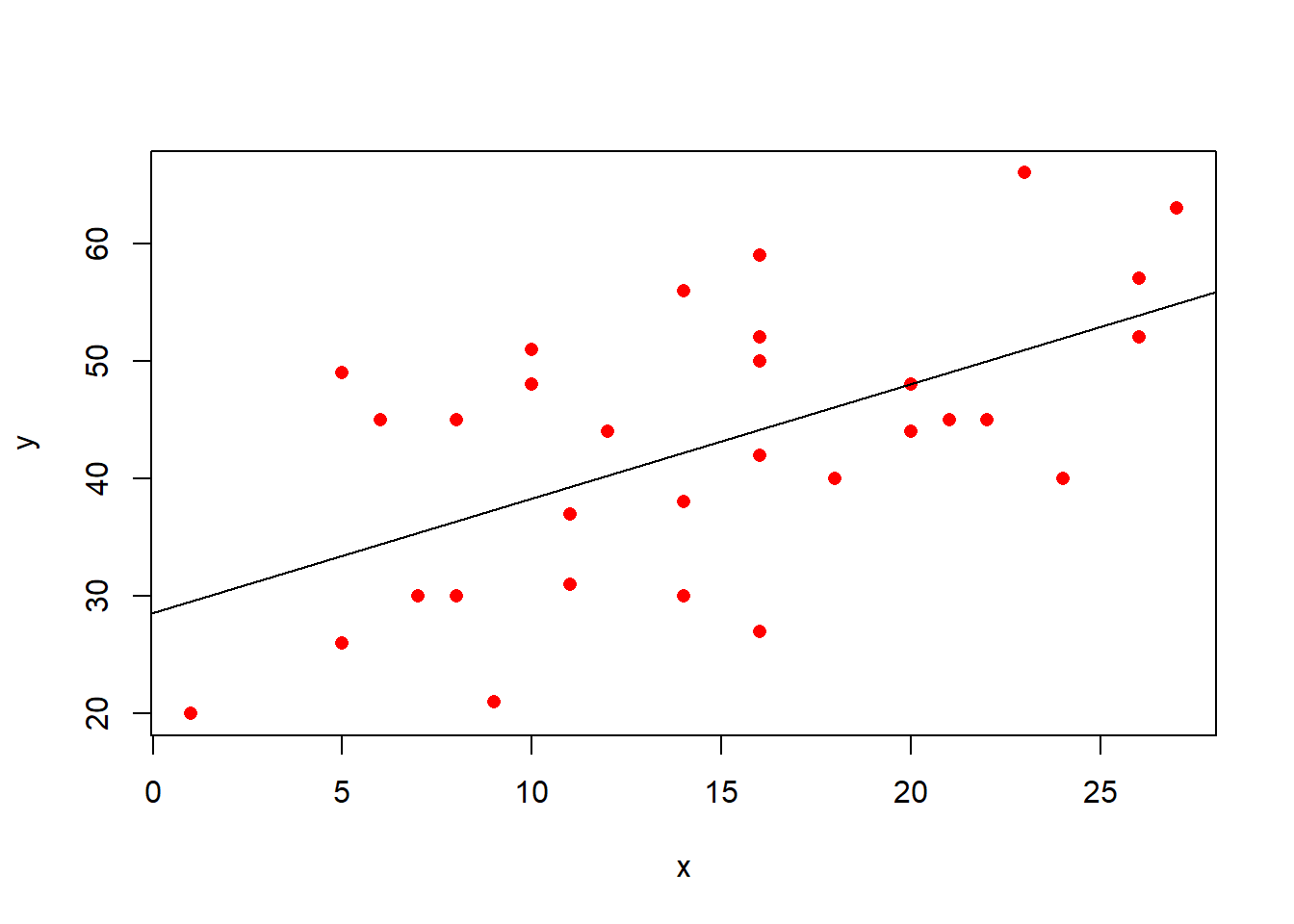
For instance, even if our outcome is the “sleep quality rating” from our class survey, measured in whole numbers from 0 to 100, our model predictions will be values that are much more specific, and my model predicted sleep quality might be 36.54374. This is because we are modelling a continuous line through the sleep quality ratings. This also means that the model extends to scores of from negative to positive infinity (\(- \infty < y < \infty\)), even though we know our scale is bounded at 0 and 100 (see Figure 2).

Often, this is a perfectly acceptable thing to do, especially when we consider the outcome variable to be measuring a continuous thing (e.g. sleep quality), just hindered by the precision of measurement, and when the bounds of our measurement tool are not preventing us from capturing variation (e.g. if everyone rates sleep as 100, there is no variance to explain).

Code

library(tidyverse)
library(patchwork)
usmr <- read_csv("https://uoepsy.github.io/data/usmr2022.csv")
ggplot(usmr, aes(x = loc, y = sleeprating)) +
  geom_point() + 
  geom_smooth(method=lm) + 
  labs(title="our model") +
  
ggplot(usmr, aes(x = loc, y = sleeprating)) +
  geom_point() + 
  geom_smooth(method=lm) + 
  geom_smooth(method=lm, se = FALSE, fullrange = TRUE) + xlim(-50,50) + 
  labs(title = "our model (zoomed out)")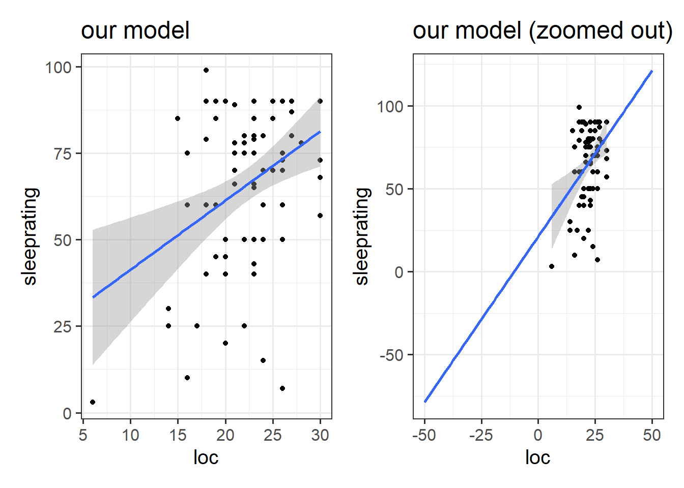

Figure 2: Our sleep quality ~ loc model is a continuous line extending infinitely

Other outcomes

There are lots of variables that we collect that don’t fit with this way of thinking. For instance, what if we want to model something that takes the form of a binary variable:¹.

• being Y vs not being Y
  
• Y happening vs Y not happening

For binary variables, values can only take one of two values, which we often encode as 0 or 1. Values can’t be 0.5, -2, or 1.3, they can only be 0 or 1.

Another type of outcome that we can’t really model as continuous is count variable:

• The number of Y’s
• How many times Y happened

For count data, values can’t take any real number, they can only take integers (0, 1, 2, 3, …).

An example

At a lake, I survey 120 people who have just finished fishing for the day. I’m interested in how the length of time they spent fishing is associated with:

1. how tired they are from 0 to 100 (continuous)
2. catching any fish (binary, 1 = yes, 0 = no)
3. the number of fish caught (count)

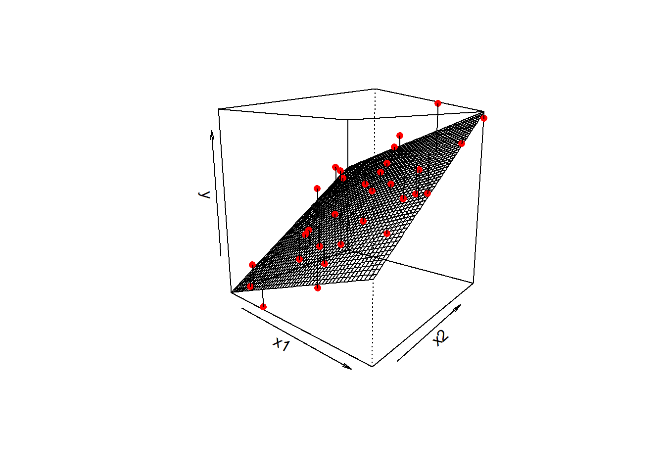
We can try at first to visualise all these relationships as scatterplots (Figure 3).

We can happily model our first outcome, tiredness, with a linear model. In Figure 3 (top panel), we can see that the relationship looks linear, and the residuals are spread fairly consistently above and below the fitted line.

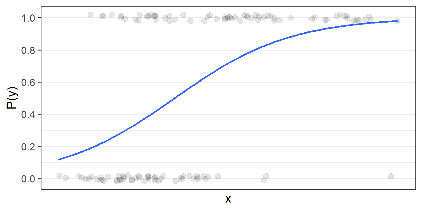
For the binary outcome however (middle panel), there are a couple of things that are problematic. For someone who spends 8 hours fishing, the model estimates approximately 1.1 “catching any fish”. But what does that 1.1 really mean? Does it mean that if I fish 8 hours I will have 1.1 fish? no, because it’s not a count. Does it mean there is a 110% probability of catching fish? This is closer, but again it doesn’t make much sense - how can we have a probability of 115%?

For the count variable (bottom panel), we can also see that the standard lm model looks problematic. Again it estimates values we simply cannot have (it looks like if i spend 1 hour fishing I will catch about negative 3 fish?). Another thing to note is that the variance in the points on the y axis tends to increase as we get higher. This is typical of count data - we’re going to see lots of people catching 0, 1 or 2 fish, and so the “people catching few fish” are all quite close (in number of fish) to one another, but because fewer people catch 20 fish, 30 fish etc, there is a lot more variability in “number of fish” when we get higher up. This is a problem for a linear model, which assumes constant variance across the fitted model.

Code

fish <- read_csv("https://uoepsy.github.io/data/fishing_exped.csv")

p1 <- ggplot(fish, aes(x = hours, y = tiredness)) + 
  geom_point() +
  labs(title="How tired are you (0 - 100)") +
  geom_smooth(method=lm, se=FALSE)

p2 <- ggplot(fish, aes(x = hours, y = caught_any)) + 
  geom_point() +
  labs(title="Did you catch any fish?") +
  geom_smooth(method=lm, se=FALSE) + 
  scale_y_continuous(limits=c(0,1.2),breaks=seq(0,1.2,.2))
  
p3 <- ggplot(fish, aes(x = hours, y = n_fish)) + 
  geom_point() +
  labs(title="How many fish did you catch?") + 
  geom_smooth(method=lm, se=FALSE)
  
p1 / p2 / p3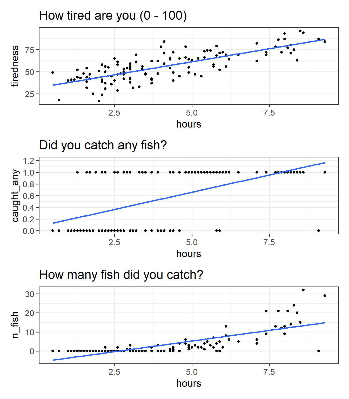

Figure 3: Three different outcomes: continuous (top), binary (middle), count (bottom)

Introducing the GLM

To deal with these sorts of outcome variable, we need to learn about the Generalised Linear Model (GLM).

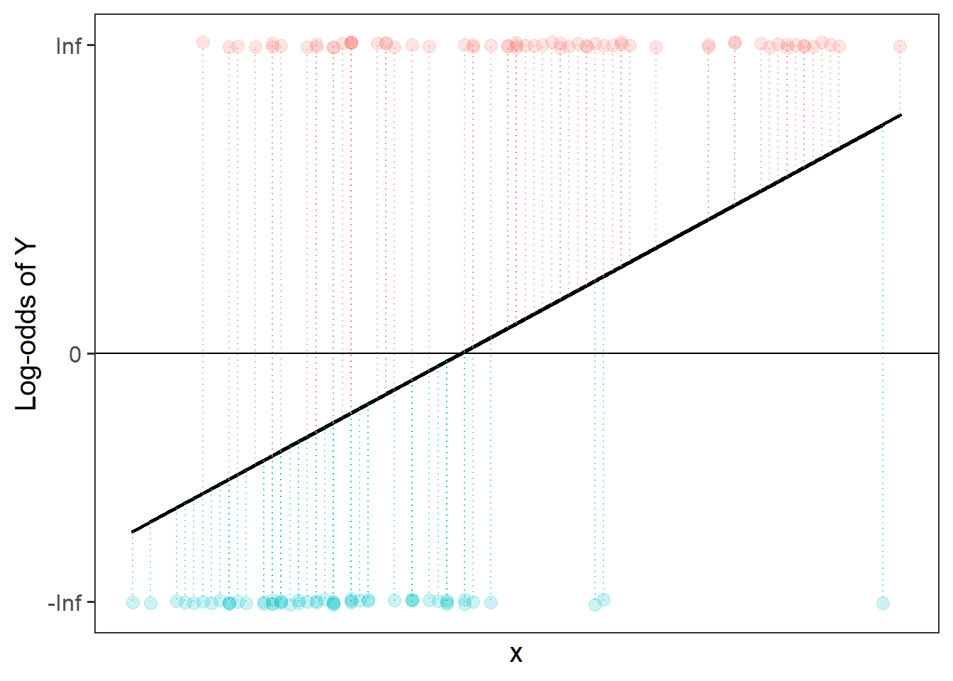
The GLM involves a little bit of trickery, in which we translate something that is inherently not linear (e.g. the probability of Y, or the increase in numbers of Y) into something which is both linear and unbounded, and model that instead.

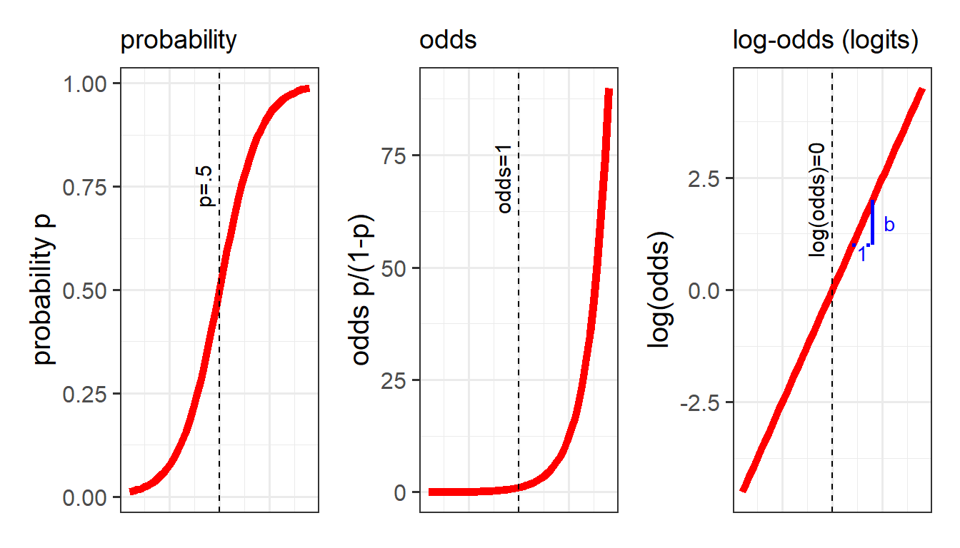
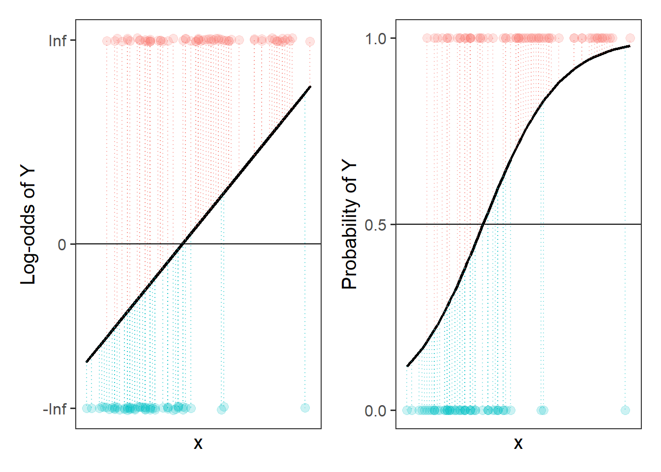
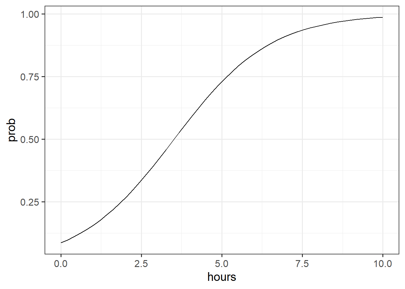
The problem, fundamentally, is that probability is not linear. We think of it as getting ever and ever closer, but never reaching - 0 and 1 (Figure 4)

Figure 4: As x increases, probability of y gets closer and closer (but never meets) 1

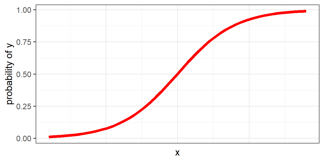
To use our linear toolbox for probability, we can’t think in terms of modelling how \(x\) influences the probability of \(y\) directly, but we can model it in terms of how it influences the “log-odds of \(y\)”. The same is true for count data: instead of modelling counts directly, we can model the log of the counts.

Probability, odds, and log-odds

If we let \(p\) denote the probability of a given event, then:

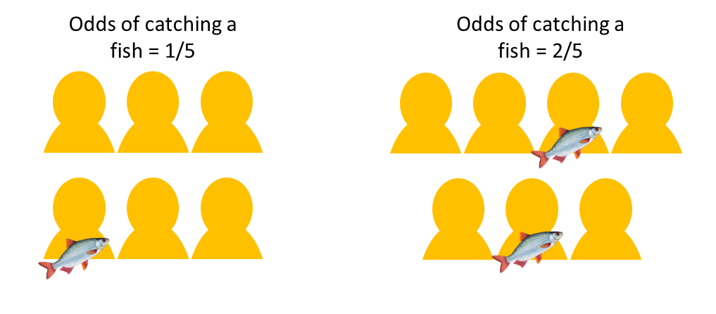
• \(\frac{p}{(1-p)}\) are the odds of the event happening.
  For example, the odds of rolling a 6 with a normal die is 1/5 (sometimes this is expressed ‘1:5’, and in gambling the order is sometimes flipped and you’ll see ‘5/1’ or ‘odds of five to one’).
  If we ever need to convert between the two:
  • \(odds = \frac{p}{(1-p)}\)
    
  • \(p = \frac{odds}{1 + odds}\)
    
• \(ln(\frac{p}{(1-p)})\) are the log-odds of the event.

Figure 5: Probability, Odds, and Log-Odds

Conversions

Between probabilities, odds and log-odds (“logit”):

$$ \[\begin{align} &\text{for probability of Y for observation i:}\\ \qquad \\ odds_i & = \frac{p_i}{1-p_i} \\ \qquad \\ logit_i &= log(odds_i) = log(\frac{p_i}{1-p_i}) \\ \qquad \\ p_i & = \frac{odds_i}{1 + odds_i} = \frac{e^{logit_i}}{(1+e^{logit_i})} \end{align}\] $$

Counts and log-counts
We can apply the same log transformation to count data in order to think about how we might consider an association on a linear

Figure 6: counts and log(counts)

Optional: What are logarithms?

Essentials of logarithms

A logarithm is a mathematical way to write any positive number as a power of a “base number”.

Log base 10

Consider the base number 10. The R function implementing the logarithm base 10 is log10().

• To what power do I need to raise the base number 10 in order to obtain the desired number 100?

x <- 100  # 100 = 10^2
x

[1] 100

pow <- log10(x)
pow

[1] 2

log10(100) = 2 as we need to raise 10 to the power of 2 in order to obtain the desired number 100.

• To what power do I need to raise the base number 10 in order to obtain the desired number 1000?

x <- 1000  # 1000 = 10^3
x

[1] 1000

pow <- log10(x)
pow

[1] 3

log10(1000) = 3 as we need to raise 10 to the power of 3 in order to obtain the desired number 1000.

Note that you can use this to write any desired number as a power of 10. For example, to which power do we raise 10 in order to obtain 13.5?

x <- 13.5
x

[1] 13.5

pow <- log10(x)
pow

[1] 1.130334

In fact, 10^1.130334 = 13.5 (up to rounding error)

10^pow

[1] 13.5

An important property is that:

\[10^{\log_{10}(x)} = x\]

For example, \(10^{\log_{10}(100)} = 10^{2} = 100\).

10^log10(100)

[1] 100

Log base e (aka natural logarithm)

A special number in mathematics is Euler’s (or Napier’s) number \(e = 2.718282\). As well as a logarithm in base 10, telling us which power to raise the base 10 to, in order to obtain a desired number, we can also use any other bases such as \(e\).

In R, you obtain Euler’s number as follows:

e <- exp(1)  # obtain the e number
e

[1] 2.718282

The logarithm with base number \(e\) is implemented in the R function log().

• To which number do I need to raise \(e\) in order to obtain 8?

x <- 8
x

[1] 8

pow <- log(8)
pow

[1] 2.079442

e^pow

[1] 8

Up to rounding error, you see that you get 8 back.

To not have rounding errors, save the full result:

pow <- log(8)
e^pow

[1] 8

An important property is that:

\[e^{\log(x)} = x\]

e^log(8)

[1] 8

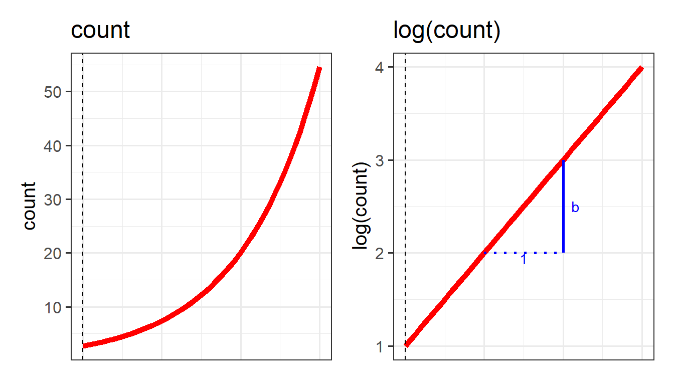
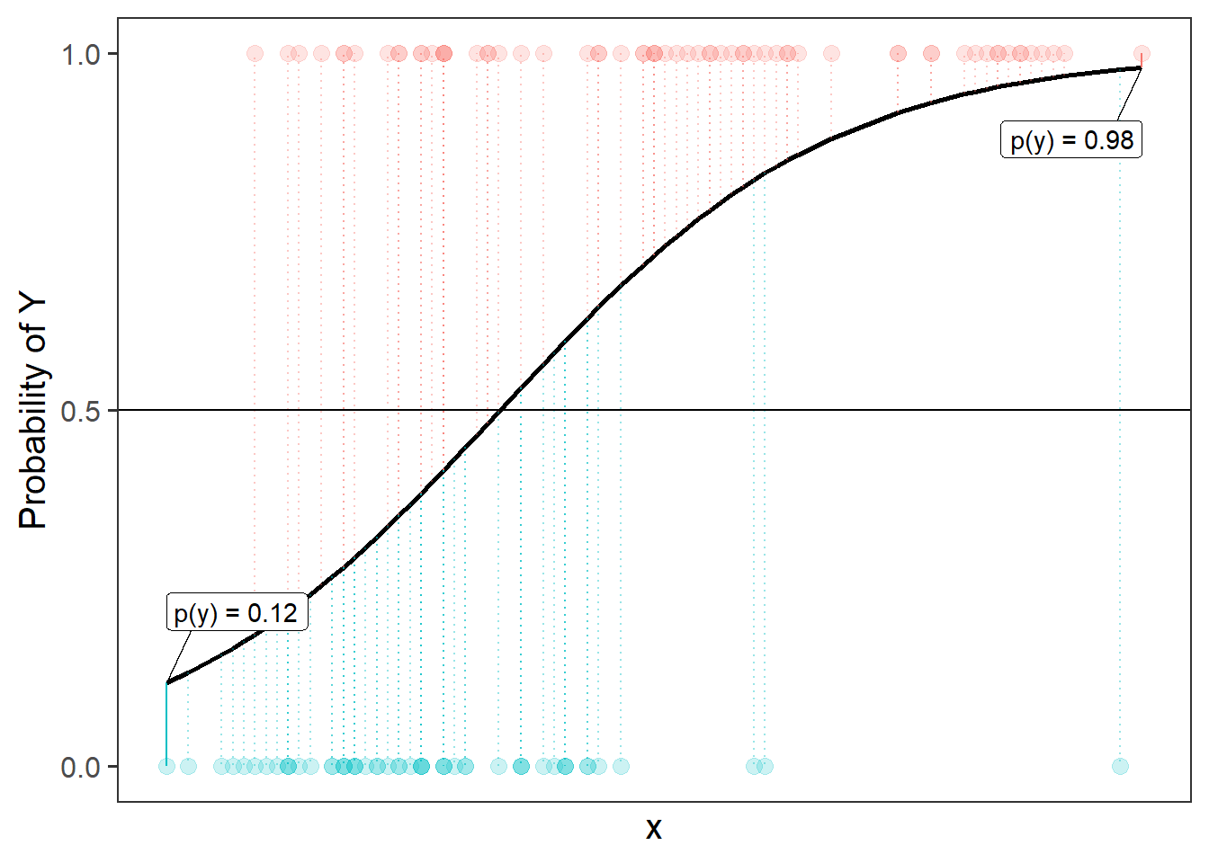
This little trick allows us to be able to talk about linear associations between predictors and the log-odds of an event, or between predictors and log-counts. In Figure 5, and Figure 6 above, we can see that by talking in terms of log-odds, or log-counts, we can model something that is linear and unbounded. So when we think about these models, what we are really have in mind is that we are capturing the associations seen in the right hand plots of Figure 5 and Figure 6.

The Generalised Linear Model

In its general form, the GLM looks pretty similar to the standard LM.
we can write it as:

\[ \color{green}{g(\color{red}{y})} = \mathbf{\color{blue}{b_0 + b_1(x_1) + ... + b_k(x_k)} } \]

The difference is that \(\color{green}{g}\) is a function (like log, or logit) that links the expected value of \(\color{red}{y}\) to the linear prediction of \(\color{blue}{b_0 + b_1(x_1) + ... + b_k(x_k)}\).

Fitting GLM in R

In order to fit these models in R, we need to use the glm() function. This is (unexpectedly) a generalised form of the lm() function we have been using. The only difference is that we need to also tell the function the family of the response variable, and the “link function” (the mapping we use to get from the thing we want to model to the thing we actually model, e.g. "log", or "logit" (log-odds)).

Linear Regression
Outcome \(y\) is continuous \(y \in (-\infty, \infty)\)

\[ \color{red}{y} = \mathbf{\color{blue}{b_0 + b_1(x_1) + ... + b_k(x_k)}} \]

linear_model <- lm(continuous_y ~ 1 + x1 + ... xk, data = df)

As it happens, lm() is just a special case of this, where we use the “gaussian” family (Gaussian is another term for ‘normal’), with the “identity” link function (the identity function is just saying ‘model y directly’):

glm(continuous_y ~ 1 + x1 + ... xk, data = df,
   family = gaussian(link = "identity"))

Logistic Regression
Outcome \(y\) is binary, \(y \in [0,1]\)

\[ \begin{align} \color{red}{ln \left( \frac{p}{1-p} \right) } &= \mathbf{\color{blue}{b_0 + b_1(x_1) + ... + b_k(x_k)}} \\ \qquad \\ \text{where } \color{red}{p} &= \text{probability of event }y\\ \end{align} \]

logistic_model <- glm(binary_y ~  1 + x1 + ... xk, data = df,
                      family=binomial(link="logit"))

• family = binomial and family = "binomial" will also work.
• the outcome can either be 0s and 1s, or coded as a factor with 2 levels.

Binomial? Binary?

The “binomial” distribution, which is used to represent the number of successes in a sequence of \(n\) independent trials (e.g. number of heads in 20 coin-flips follows a binomial distribution, see Lecture 4!).
A binary response is a special case of this, where \(n = 1\).

The logistic regression model, more generally, can be written as:

\[ \begin{align} \color{red}{ln \left( \frac{p}{1-p} \right) } &= \mathbf{\color{blue}{b_0 + b_1(x_1) + ... + b_k(x_k)}} \\ \qquad \\ \text{where } Y &\sim Binomial(n, \color{red}{p})\\ \end{align} \]

Poisson Regression
Outcome \(y\) is positive \(y \in (0, \infty)\)

\[ \color{red}{ln (y) } = \mathbf{\color{blue}{b_0 + b_1(x_1) + ... + b_k(x_k)}} \]

poisson_model <- glm(count_y ~  1 + x1 + ... xk, data = df,
                     family=poisson(link="log"))

• family = poisson and family = "poisson" will also work

Optional: A tangent: Model estimation

Maximum Likelihood Estimation

For a linear regression, R has been fitting our regression models by “minimising the residual sums of squares” (i.e., we rotate the line to find the point at which \(\sum{(y - \hat{y})^2}\) is smallest. This gave us the “best fitting line” (Figure 7).

Figure 7: https://uoepsy.github.io/usmr/2223/lectures/lecture_7.html#34

For the generalized linear models we can’t do this. For instance, in logistic regression model, what we’re really wanting is the “best fitting squiggle” (Figure 8), and to get to this we must do something else other than looking at our residuals \(y - \hat{y}\).

Figure 8: Probability of Y across values of X

The reason we have to do something different is because for our actual observations, the event has either happened or it hasn’t. So we can’t take the raw data as “probabilities” which we can translate into log-odds. We can try, but it doesn’t make sense, and we would just be trying to fit some line between infinity and negative infinity (Figure 9). This would mean the residuals would also all be infinity, and so it becomes impossible to work out anything!

# A tibble: 3 × 3
  observed odds  log_odds
  <chr>    <chr> <chr>   
1 0        0     -Inf    
2 1        Inf   Inf     
3 ...      ...   ...     

Figure 9: In the log-odds world, comparing our predicted values to observed values of -Inf and Inf isn’t very useful, because all those distances will be infinite (there is no way of measuring the dotted lines, so we can’t really use them)

Instead, maximum likelihood estimation is used to find the set of coefficients which best reproduce the observed data.
To do this, the computer considers loads of different lines, trying to slowly converge on the one which increases the likelihood of the data.

To understand this a bit better, let’s take consider one possible line in the probability world. The left-hand plot of Figure 10 is the same line as the one shown in Figure 9, and we can see it translated back into probabilities in the right-hand plot, so that we have a predicted probability of the outcome for each datapoint. From the right-hand plot, we can then ask “what is the likelihood of the data, given this line?”. To get this, we multiply up all the probabilities that observed 1s are predicted as 1s and that observed 0s predicted as 0s.

Figure 10: Note - the dotted lines are not residuals, but just to show the projections of observations down to the line

As an example Figure 11 shows the predicted probabilities for a couple of datapoints. The furthest left point is an observed 0, and so the likelihood of this data given the predicted probability is 1-0.12, or 0.88. The furthest right is an observed 1, so the likelihood of this is 0.98. This means the probability of seeing those two datapoints, given the line we have, is 0.98 * 0.88. But what we want is the probability of seeing all our data, given this line. So we need to do this for all of the datapoints.² Once we have this, we can compare the likelihood of all of seeing this data for a whole range of different lines.

The cool thing is that computers do all this for us. Maximum likelihood estimation is just a method to find out which parameters maximise the likelihood of the data. In our context, it tells us what values of coefficients in \(\color{red}{ln\left(\frac{p}{1-p} \right)} = \color{blue}{\beta_0 \cdot{} 1 + \beta_1 \cdot{} X_1 }\) maximise the likelihood of reproducing the data we observed.

Figure 11: Note - the dotted lines are not residuals, but just to show the projections of observations down to the line

Logistic Regression

For the remainder of this reading, we’re going to leave discussions of Poisson regression and focus on working with binary outcomes using logistic regression, which you are much more likely to encounter in your reading/research. A lot of the logic of these models transfers across to when we work with count data, but you will not need poisson regression for any assignment on this course.

Let’s return to our fishing example, and fit a model in which we predict “having caught some fish” by the number of hours spent fishing.

Practically, speaking, this quite straightforward. We have a binary outcome (1 = caught fish, 0 is didn’t catch fish), so we’ll fit a logistic regression. We have a single predictor, which is “hours spent fishing”:

fish <- read_csv("https://uoepsy.github.io/data/fishing_exped.csv")
fishmod <- glm(caught_any ~ hours, data = fish,
               family = binomial(link="logit"))
summary(fishmod)

Call:
glm(formula = caught_any ~ hours, family = binomial(link = "logit"), 
    data = fish)

Deviance Residuals: 
    Min       1Q   Median       3Q      Max  
-2.7450  -0.8866   0.2910   0.8161   1.8381  

Coefficients:
            Estimate Std. Error z value Pr(>|z|)    
(Intercept)  -2.3567     0.5322  -4.428 9.50e-06 ***
hours         0.6704     0.1377   4.870 1.12e-06 ***
---
Signif. codes:  0 '***' 0.001 '**' 0.01 '*' 0.05 '.' 0.1 ' ' 1

(Dispersion parameter for binomial family taken to be 1)

    Null deviance: 165.15  on 119  degrees of freedom
Residual deviance: 127.70  on 118  degrees of freedom
AIC: 131.7

Number of Fisher Scoring iterations: 5

Interpretation of Coefficients

An important result of our model capturing the linear associations between the predictors and the log-odds of outcome Y, is that our coefficients are all in these units.

summary(fishmod)

Call:
glm(formula = caught_any ~ hours, family = binomial(link = "logit"), 
...
Coefficients:
            Estimate Std. Error z value Pr(>|z|)    
(Intercept)  -2.3567     0.5322  -4.428 9.50e-06 ***
hours         0.6704     0.1377   4.870 1.12e-06 ***

• (Intercept): the log-odds of having caught some fish when spending zero hours fishing are -2.36.
  
• hours coefficient: for every hour someone has spent fishing, the log-odds of them having caught some fish increase by 0.67.

If you’re anything like me, these are not the most useful interpretations. I have no idea what increasing 0.67 log-odds means in real terms. What we can do instead is translate these back into odds, which might make things easier. The opposite of the natural logarithm is the exponential (see here if you’re interested). We can turn \(log(x)\) back into \(x\) by raising \(e\) to the power of it: \(e^{\log(x)} = x\). In R, this is just the two functions log() and exp(): exp(log(2)) == 2.

This means we can turn our log-odds back into odds by using exp() on our coefficients! A crucial thing to note is that addition on the log-odds scale is the same as multiplication on the odds scale. A coefficient on the log-odds scale is interpreted the same way as we interpret normal linear regression coefficients: “if you go up 1 on X you add b on log-odds(Y)”. When we convert these coefficients to odds using exp(), the interpretation becomes “if you go up 1 on X, your odds are multiplied by exp(b)”.

We can see our exponentiated coefficients here:

exp(coef(fishmod))

(Intercept)       hours 
 0.09473306  1.95504622 

The intercept is now the odds of having caught a fish when spending zero hours fishing: 0.09.

Because our intercept is at a single point (it’s not an association), we can actually convert this to a probability. Remember that \(odds = \frac{p}{1-p}\), which means that \(p = \frac{odds}{1 + odds}\). So the probability of catching a fish if I spend zero hours fishing is \(\frac{0.09}{1 + 0.09} = 0.08\).

Unfortunately, we can’t do the same for any of the slope coefficients. This is because changes in odds are not the same for different levels of probability.

quick demonstration

Consider how when we multiply odds by 2, the increase in probability is not constant:

Odds	Probability
0.5	\(\frac{1}{1+0.5} = 0.33\)
1	\(\frac{1}{1+1} = 0.5\)
2	\(\frac{2}{1+2} = 0.66\)
4	\(\frac{4}{1+4} = 0.8\)
8	\(\frac{8}{1+8} = 0.88\)

Our best interpretation of our coefficient for hours is simply that for every hour someone has spent fishing, the odds of them having caught some fish are multiplied by 1.96.

Odds Ratios

When we exponentiate coefficients from a model fitted to the log-odds, the resulting association is referred to as an “odds ratio” (OR).

For every 1 unit increase in \(x\):

• “the odds of \(y\) change by a ratio of exp(b)”
  
• “the odds of \(y\) are multiplied by exp(b)”
  
• “there are exp(b) increased/decreased odds of \(y\)”

Instead of thinking of a coefficient of 0 as indicating “no association”, in odds ratios this when the OR = 1.

• OR = 1 : equal odds (\(1 \times odds = odds \text{ don't change}\)).
• OR < 1 : decreased odds (\(0.5 \times odds = odds \text{ are halved}\))
• OR > 1 : increased odds (\(2 \times odds = odds \text{ are doubled}\))

Often you will hear people interpreting OR as “\(y\) is exp(b) times as likely to occur”.
Although it is true that increased odds is increased likelihood of \(y\) occurring. Double the odds does not mean you will see twice as many occurrences of \(y\) (see the “I still don’t really get odds” box below).

I still don’t really get odds..

Even talking in odds and multiplying odds can be frustratingly confusing, so here’s a little more step-by-step explanation to try and help:

term	b	exp(b)
(Intercept)	-2.36	0.09
hours	0.67	1.96

1. For people spending just 1 hour fishing, the log-odds of them having caught fish are -2.36 + 0.67 = -1.69.
   
2. Translating this to odds, we exponentiate it, so the odds of them having caught fish are \(e^{(-2.36 + 0.67)} = e^{-1.69} = 0.19\).
   (This is the same³ as \(e^{-2.36} \times e^{0.67}\))
   
3. These odds of 0.19 equate to approximately \(\frac{1}{5}\), which means that if we take 6 people who have each spent 1 hour fishing, we expect 1 of them to have caught fish, and 5 of them to have not caught anything.
   
4. If we consider how the odds increase for every hour spent fishing (i.e. for those spending 2 hours fishing as opposed to just 1):
   • the log-odds of catching fish increase by 0.67.
     
   • the odds of catching fish are multiplied by 1.96.
     
   • so for 2 hours of fishing, the odds are \(0.19 \times 1.96 = 0.36\).
     (And we can also calculate this as \(e^{-1.69 + 0.67}\))
     
5. So these new odds of 0.36 for 2 hours fished are 1.96 times greater than the odds of 0.19 for 1 hour fished. For ease, let’s just round 1.96 to 2 and say that the odds have doubled.
   What does this mean? It means we’ve gone from odds of \(\frac{1}{5}\) to \(\frac{2}{5}\). This doesn’t mean we’ll now see 2 out of 6 people catching fish. It means we’ll see 2 out of 7 (Figure 12).

Figure 12: Increasing from odds of 1/5 to 2/5

Inference

Coefficient Tests

You might notice that the summary output of our logistic regression model has \(z\) statistics instead of \(t\) statistics. For logistic regression, the distribution of the estimated coefficients gets close and closer to a Normal distribution as the sample size gets larger. All of the tests are based on the hypothesis that the sample size is large enough⁴ to justify a normal approximation.

summary(fishmod)

Coefficients:
            Estimate Std. Error z value Pr(>|z|)    
(Intercept)  -2.3567     0.5322  -4.428 9.50e-06 ***
hours         0.6704     0.1377   4.870 1.12e-06 ***

The logic of the tests remains the same as it was for the linear model, where it is a test against the null hypothesis that the coefficient is zero. Or, less formally, we can think of the corresponding p-value as “in the null universe where there is no relationship between \(x\) and the occurrence of event \(y\), there is a p-value chance of seeing a sample of this size with an association as strong as the one we have got”

For every hour more someone spent fishing, the odds of them catching a fish increased by 1.96 (\(z = 4.87\), \(p < .001\)).

Confidence Intervals
As previously, we can obtain confidence intervals using the confint() function. Because confidence intervals are just lower and upper bounds for a range of plausible values for our estimates, we can turn these into the confidence intervals around our odds ratios!

exp(confint(fishmod))

                 2.5 %    97.5 %
(Intercept) 0.03102087 0.2534272
hours       1.52614259 2.6275396

For every hour more someone spent fishing, the odds of them catching a fish increased by 1.96 (95% CI [1.53, 2.63]).

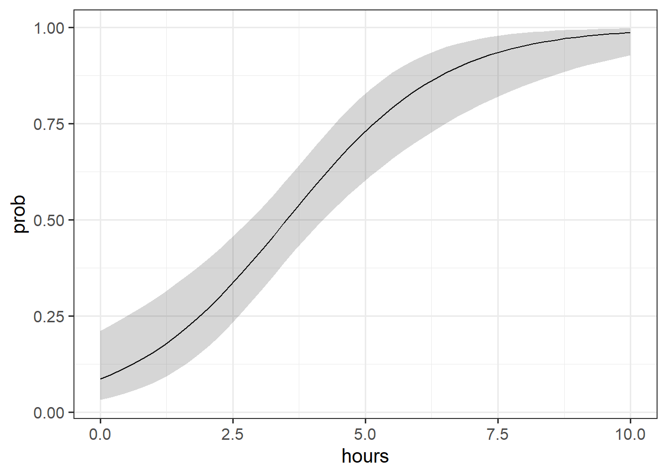
Visualising

While interpreting coefficients leaves us in speaking in the realm of odds-ratios, we can do more with visualisations! This is because we can simply display the predicted probability across values of some predictor. We don’t have to try and rely solely on a numerical description of a relationship - a picture speaks a thousand words (and it’s a lot easier!)

library(sjPlot)
plot_model(fishmod, type = "eff")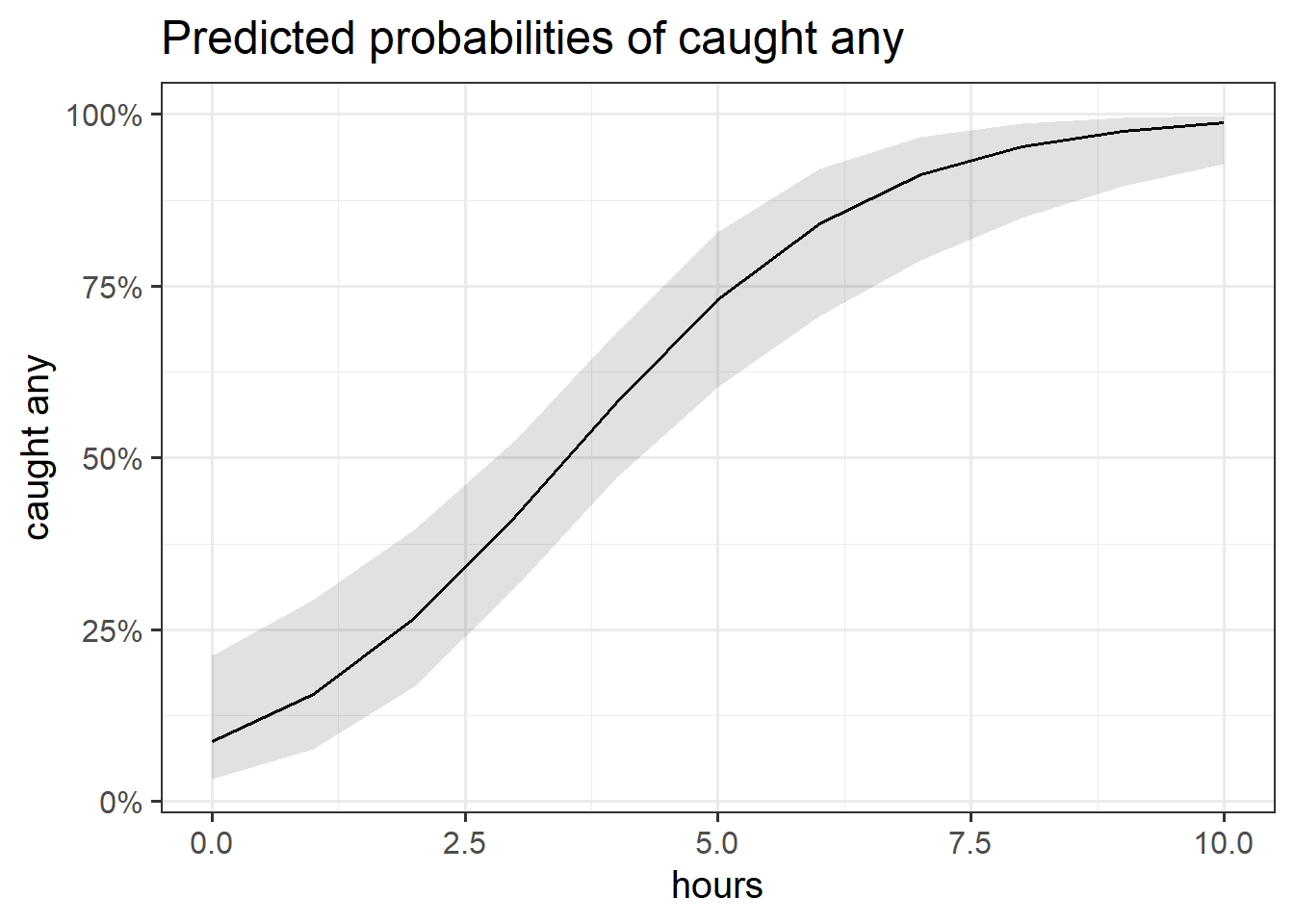

$hours

Optional: making plots manually

to make plots manually, we need to give our model some new data to predict values for, and then plot those predictions!
For these models, we can actually predict on various different scales (e.g. do we want to predict log-odds values (predict(mod, type="link")) or probabilities (predict(mod, type="response"))?

plotdata <- tibble(
  # make hours a sequence of length 50, from 0 to 10
  hours = seq(0, 10, length.out = 50)
)

# add the predcted probabilities
plotdata <- 
  plotdata %>% mutate(
    prob = predict(fishmod, newdata = plotdata, type = "response"),
  )

# plot the predicted probabilities
ggplot(plotdata, aes(x = hours, y = prob)) +
  geom_line()

# Getting the intervals is much trickier, but essentially requires computing the upper and lower bounds on the log-odds scale and then converting them back:
plotdata <- 
  plotdata %>% 
  mutate(
    logodd = predict(fishmod, newdata = plotdata, type = "link"),
    se = predict(fishmod, newdata = plotdata, type = "link", se.fit = TRUE)$se,
    logoddlower = logodd - (1.96*se),
    logoddupper = logodd + (1.96*se),
    prob = fishmod$family$linkinv(logodd),
    lower = fishmod$family$linkinv(logoddlower),
    upper = fishmod$family$linkinv(logoddupper)
  )

ggplot(plotdata, aes(x = hours, y = prob)) +
  geom_line() + 
  geom_ribbon(aes(ymin=lower,ymax=upper), alpha=.2)

Comparing models

When moving from linear regression to more advanced and flexible models, testing of goodness of fit is more often done by comparing a model of interest to a simpler one. The only caveat is that the two models need to be nested, i.e. one model needs to be a simplification of the other, and all predictors of one model needs to be within the other.

To compare models, we test the difference in deviance.

Deviance

Deviance is a measure of deviation/discrepancy/mismatch between the data and the model. You can think of it as a generalisation of the terms making up the residual sum of squares in simple linear regression, in that it measures the misfit, or badness of fit. This means (as it was for the residual sum of squares) that smaller deviance is better!

More technically, deviance is calculated as -2 times the log-likelihood.

• Likelihood = \(P(data | model)\) (the probability of seeing the sample data given our model). If we had a perfect model, this would be 1.
  • if you want a (slightly) more in depth look at “likelihood”, see here.
• Log-likelihood = the log of the likelihood. The log transformation means that where likelihood ranges from 0 to 1, log-likelihood ranges from negative infinity to 0 (0 would be the perfect model)
• -2Log-likelihood = turns it from negative to positive, and allows us to test it against a \(\chi^2\) distribution.

For instance, we can compare our model to the model where all slopes are 0. The null hypothesis will be that the simpler model is a good fit, while the alternative is that the more complex model is needed.

In R we do this comparison as follows:

fishmod0 <- glm(caught_any ~ 1, data = fish,
               family = binomial(link="logit"))

fishmod1 <- glm(caught_any ~ hours, data = fish,
               family = binomial(link="logit"))

anova(fishmod0, fishmod1, test = 'Chisq')

Analysis of Deviance Table

Model 1: caught_any ~ 1
Model 2: caught_any ~ hours
  Resid. Df Resid. Dev Df Deviance  Pr(>Chi)    
1       119     165.15                          
2       118     127.70  1    37.45 9.378e-10 ***
---
Signif. codes:  0 '***' 0.001 '**' 0.01 '*' 0.05 '.' 0.1 ' ' 1

The above code shows the two fitted models, amd reports the Residual Deviance of each model, 165.1 and 127.7 respectively. So by adding the predictor hours to the model, we reduce our deviance from 165.1 to 127.7, i.e. we reduce it by 37.4 (remember, deviance is like badness-of-fit, so smaller is better).
Is this reduction sufficient to be attributed solely to the contribution of the predictor, or could it just be due to random sampling variation? This is what the chi-squared test tells us!

Optional Akaike and Bayesian Information Criteria

Deviance measures lack of fit, and it can be reduced to zero by making the model more and more complex, effectively estimating the value at each single data point. However, this involves adding more and more predictors, which makes the model more complex (and less interpretable).

Typically, simpler models are preferred when they still explain the data almost as well. This is why information criteria were devised, exactly to account for both the model misfit but also its complexity.

\[ \text{Information Criterion} = \text{Deviance} + \text{Penalty for model complexity} \]

Depending on the chosen penalty, you get different criteria. Two common ones are the Akaike and Bayesian Information Criteria, AIC and BIC respectively:

\[ \begin{aligned} \text{AIC} &= \text{Deviance} + 2 p \\ \text{BIC} &= \text{Deviance} + p \log(n) \end{aligned} \]

where \(n\) is the sample size and \(p\) is the number of regression coefficients in the model. Models that produce smaller values of these fitting criteria should be preferred.

AIC and BIC differ in their degrees of penalization for number of regression coefficients, with BIC usually favouring models with fewer terms.

AIC(fishmod0, fishmod1)

         df      AIC
fishmod0  1 167.1533
fishmod1  2 131.7031

BIC(fishmod0, fishmod1)

         df      BIC
fishmod0  1 169.9408
fishmod1  2 137.2781

According to both AIC and BIC the model with hours as a predictor has a lower score, meaning it’s preferable to the other.

Assumptions

Because these models don’t have the same expected error distribution (we don’t expect residuals to be normally distributed around the mean, with constant variance), checking the assumptions of logistic regression is a little different.

Typically, we look at the “deviance residuals”. But we don’t examine plots for patterns, we simply examine them for potentially outlying observations. If we use a standardised residual, it makes it easier to explore extreme values as we expect most residuals to be within -2, 2 or -3, 3 (depending on how strict we feel).

Deviance Residuals

There are three ways we can get out deviance residuals, each scaled differently

• \(i\)th residual = measure of deviance contributed from the \(i\)th observation
• \(i\)th standardized residual = residual / SD(residual)
• \(i\)th studentized residual = residual / SD(residual from model fitted without observation \(i\))

We get these in R using:

# deviance residuals
residuals(fishmod, type = 'deviance')
# studentised residuals
rstudent(fishmod, type = 'deviance')
# standardised residuals
rstandard(fishmod, type = 'deviance')

We can check whether any residuals are larger than 2 or 3 in absolute value:

plot(rstudent(fishmod, type = 'deviance'), 
     ylab = 'Studentized Deviance Residuals')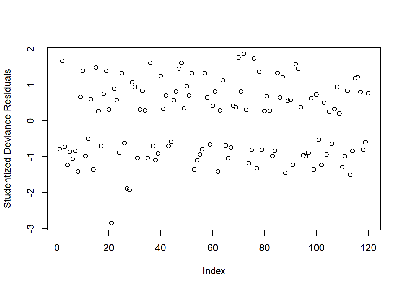

Warning: Don’t inspect this plot for patterns!!!

There appears to be 1 residual with a value slightly larger than 2 in absolute value. We will keep these in mind and check later if they are also influential points (using cooks.distance)

Sometimes a binned plot⁵ can be more informative, but not always! It works by combining together all responses for people having the same covariate \(x_i\) value, and taking the average studentized Pearson residual for those.

Before using this function, make sure you have installed the arm package!

arm::binnedplot(fitted(fishmod), rstudent(fishmod, type = 'deviance'), 
                xlab = 'Prob. of Catching fish', ylab = 'Studentized Deviance Residuals')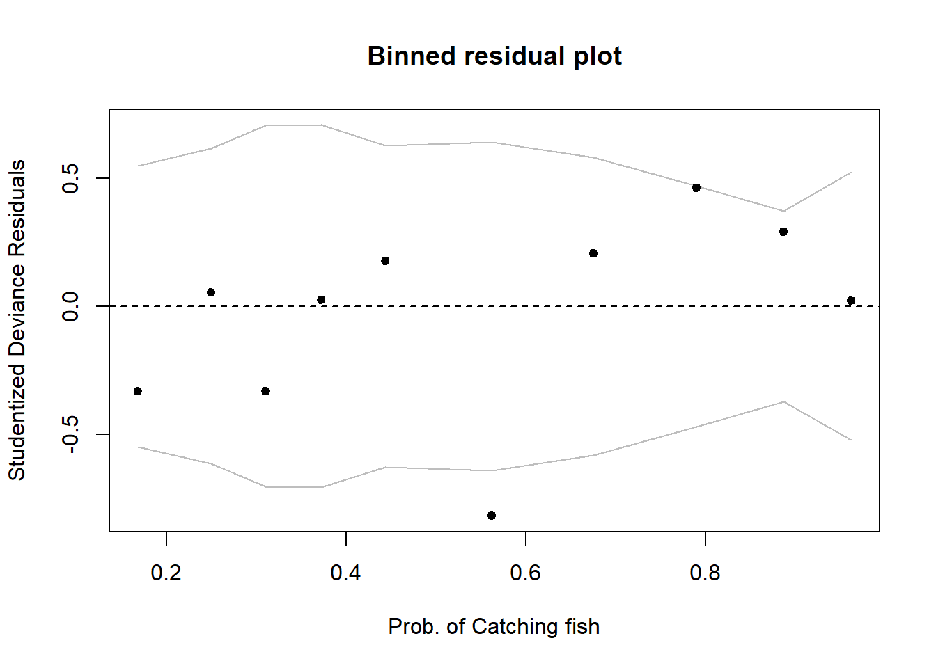

There doesn’t appear to be any extreme residuals.

Footnotes

1. we have seen this type of variable already when looking at categorical predictors in our models, but we haven’t seen how we use it as the outcome

2. This means we will end up with a lot of multiplying (computationally expensive), and a tiny tiny number. So instead we typically talk about the log-likelihood, and use summation instead of multiplication. The log-likelihood of the two data points highlighted in Figure 10, given the line is log(0.98)+log(0.88).

3. \(e^{a+b} = e^a \times e^b\). For example: \(2^2 \times 2^3 = 4 \times 8 = 32 = 2^5 = 2^{2+3}\)

4. whatever ‘large enough’ is!

5. Gelman, A., & Hill, J. (2006). Data Analysis Using Regression and Multilevel/Hierarchical Models (Analytical Methods for Social Research). Cambridge: Cambridge University Press. doi:10.1017/CBO9780511790942