Week 4 Exercises: Chi-Square Tests

Birth-Months

Research Question: Are people more likely to be born in certain months than others?

As you may remember, in the survey we asked students to complete in welcome week, one of the questions concerned the month in which you were born. You can download the data from https://uoepsy.github.io/data/surveydata_allcourse22.csv.

survey_data <- 
  read_csv("https://uoepsy.github.io/data/surveydata_allcourse22.csv")

Question 1

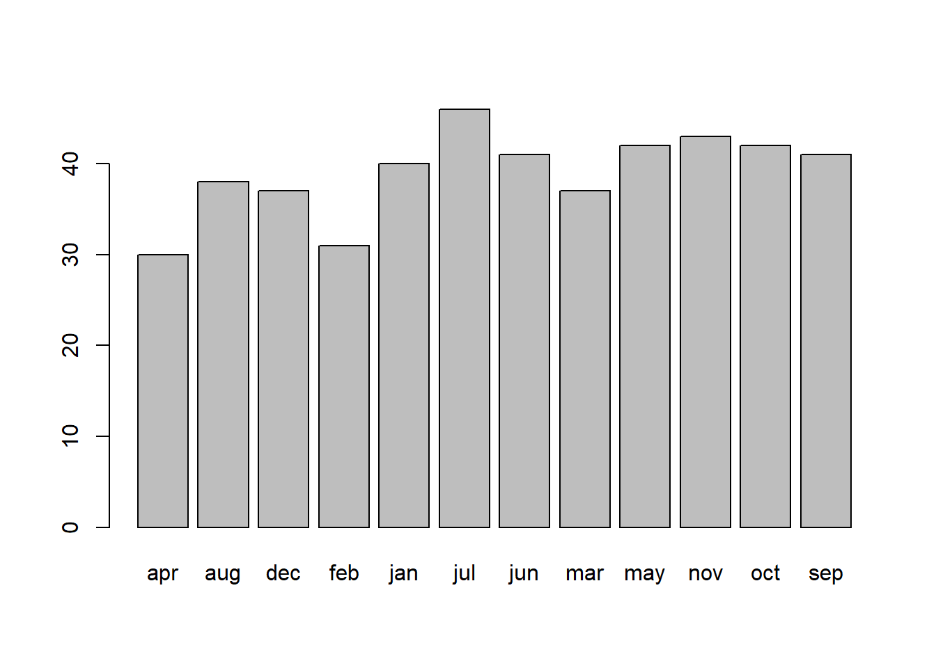
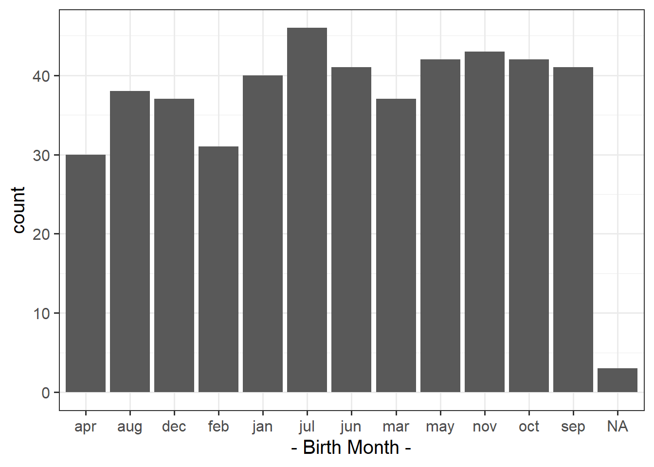
What is your intuition about the distribution of all students’ birth-months?
Do you think they will be spread uniformly across all months of the year (like a fair 12-sided dice), or do you think people are more likely to be born in certain months more than others?

Plot the distribution and get an initial idea of how things are looking.

Hint:
You can do this quickly with barplot() and table(), or you could create try using ggplot() and looking into geom_bar().

Solution

The quick and dirty way to plot:

barplot(table(survey_data$birthmonth))

A ggplot option:

ggplot(data = survey_data, aes(x = birthmonth)) +
    geom_bar() +
    labs(x = "- Birth Month -")

Question 2

We’re going to perform a statistical test to assess the extent to which our data conforms to the hypothesis that people are no more likely to be born on one month than another.

Under this hypothesis, what would be the proportional breakdown of observed births in each of the months?

Solution

If people are no more likely to be born in one month than another, then we would expect the same proportion of observed births in each month.
There are 12 months, so we would expect \(\frac{1}{12}\) observations in each month.

We can write these as:

\[ \begin{align} & p_{jan} = 1/12 \\ & p_{feb} = 1/12 \\ & ... \\ & p_{dec} = 1/12 \\ \end{align} \]

Question 3

We can find out how many people have valid entries (i.e. not NA) in the birth-month variable:

sum(!is.na(survey_data$birthmonth))

[1] 468

Given this information, how many observations would we expect to find with a birthday in January? And in February? … and so on?

Solution

We would expect \(\frac{1}{12} \times\) 468 = 39 observations in each month.

Question 4

The code below creates counts for each month. Before doing that, it removes the rows which have an NA in them for birthmonth:

survey_data %>%
  filter(!is.na(birthmonth)) %>%
  group_by(birthmonth) %>%
  summarise(
      observed = n()
  )

(A shortcut for this would be survey_data %>% filter(!is.na(birthmonth)) %>% count(birthmonth))

Add to the code above to create columns showing:

• the expected counts \(E_i\)
• observed-expected (\(O_i - E_i\))
• the squared differences \((O_i - E_i)^2\)
• the standardised square differences \(\frac{(O_i - E_i)^2}{E_i}\)

Then calculate the \(\chi^2\) statistic (the sum of the standardised squared differences).
If your observed counts matched the expected counts perfectly, what would the \(\chi^2\) statistic be?

Hint: This was all done in the manual example of a \(\chi^2\) test in 4A #chi2-goodness-of-fit-test

Solution

chi_table <- 
    survey_data %>%
    filter(!is.na(birthmonth)) %>%
    group_by(birthmonth) %>%
    summarise(
        observed = n(),
        expected = sum(!is.na(survey_data$birthmonth))/12,
        diff = observed-expected,
        sq_diff = diff^2,
        std_sq_diff = sq_diff / expected
    )
chi_table

# A tibble: 12 × 6
   birthmonth observed expected  diff sq_diff std_sq_diff
   <chr>         <int>    <dbl> <dbl>   <dbl>       <dbl>
 1 apr              30       39    -9      81      2.08  
 2 aug              38       39    -1       1      0.0256
 3 dec              37       39    -2       4      0.103 
 4 feb              31       39    -8      64      1.64  
 5 jan              40       39     1       1      0.0256
 6 jul              46       39     7      49      1.26  
 7 jun              41       39     2       4      0.103 
 8 mar              37       39    -2       4      0.103 
 9 may              42       39     3       9      0.231 
10 nov              43       39     4      16      0.410 
11 oct              42       39     3       9      0.231 
12 sep              41       39     2       4      0.103 

And we can calculate our \(\chi^2\) test statistic by simply summing the values in the last column we created:

sum(chi_table$std_sq_diff)

[1] 6.307692

If all our observed counts are equal to our expected counts, then the diff column above will be all \(0\), and \(0^2=0\), and \(\frac{0}{E_i}\) will be \(0\). So \(\chi^2\) will be \(0\).

Question 5

You can see the distribution of \(\chi^2\) statistics with different degrees of freedom below.

Figure 1: Chi-Square Distributions

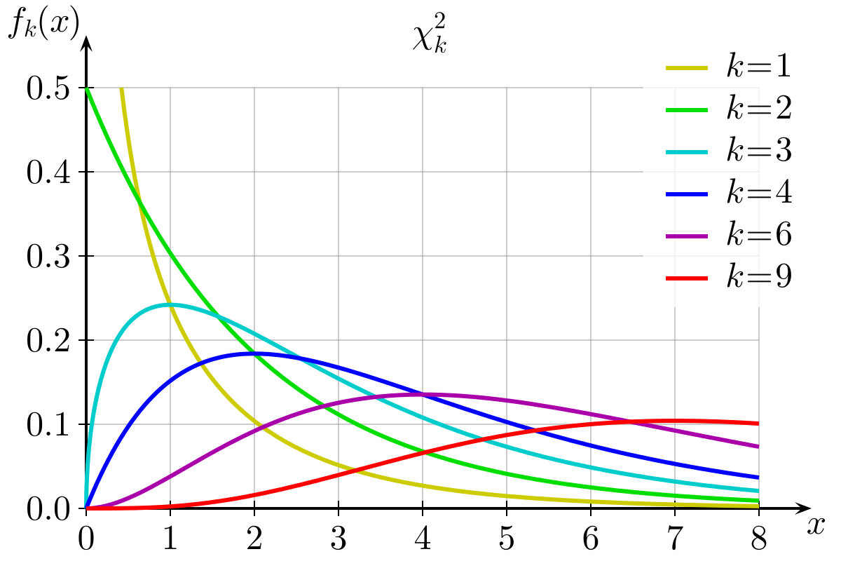
We can find out the proportion of the distribution which falls to either side of a given value of \(\chi^2\) using pchisq(). We need to give it our calculated \(\chi^2\) statistic, our degrees of freedom (df), which is equal to the number of categories minus 1. We also need to specify whether we want the proportion to the left (lower.tail=TRUE) or to the right (lower.tail=FALSE).

1. Using pchisq(), calculate the probability of observing a \(\chi^2\) statistic as least as extreme as the one we have calculated.
   
2. Check that these results match with those provided by R’s built-in function: chisq.test(table(survey_data$birthmonth)) (the table function will ignore NAs by default, so we don’t need to do anything extra for this).

Solution

sum(chi_table$std_sq_diff)

[1] 6.307692

pchisq(sum(chi_table$std_sq_diff), df = 11, lower.tail = FALSE)

[1] 0.8520656

chisq.test(table(survey_data$birthmonth))

    Chi-squared test for given probabilities

data:  table(survey_data$birthmonth)
X-squared = 6.3077, df = 11, p-value = 0.8521

Question 6

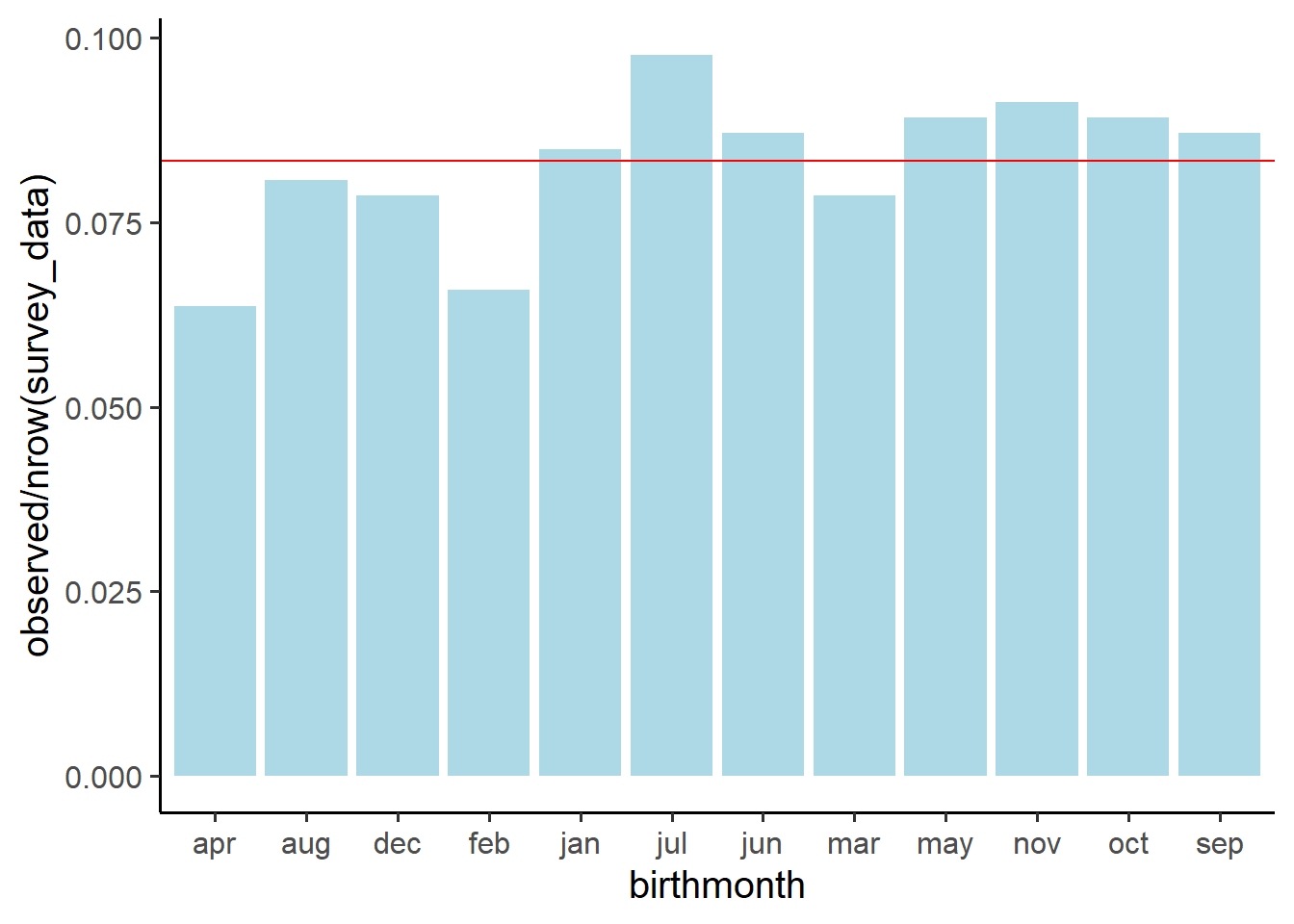
Which months of year had the highest contributions to the chi-square test statistic?

Hint: Think about your standardised squared deviations.

Solution

Standardized squared deviations

One possible way to answer this question is to look at the individual contribution of each category to the \(\chi^2\) statistic. We computed these values in an earlier question.

chi_table %>%
  select(birthmonth, std_sq_diff)

# A tibble: 12 × 2
   birthmonth std_sq_diff
   <chr>            <dbl>
 1 apr             2.08  
 2 aug             0.0256
 3 dec             0.103 
 4 feb             1.64  
 5 jan             0.0256
 6 jul             1.26  
 7 jun             0.103 
 8 mar             0.103 
 9 may             0.231 
10 nov             0.410 
11 oct             0.231 
12 sep             0.103 

From the barplot we created earlier on, we can see which months make up higher/lower proportions than expected:

ggplot(chi_table, aes(x = birthmonth, y = observed/nrow(survey_data))) +
  geom_col(fill = 'lightblue') +
  geom_hline(yintercept = 1/12, color = 'red') +
  theme_classic(base_size = 15)

Pearson residuals

Equivalently, you could answer by looking at Pearson residuals:

chisq.test(table(survey_data$birthmonth))$residuals

       apr        aug        dec        feb        jan        jul        jun 
-1.4411534 -0.1601282 -0.3202563 -1.2810252  0.1601282  1.1208971  0.3202563 
       mar        may        nov        oct        sep 
-0.3202563  0.4803845  0.6405126  0.4803845  0.3202563 

The greatest absolute values are for apr and feb, showing that for these months the deviations from expected to observed were the greatest.

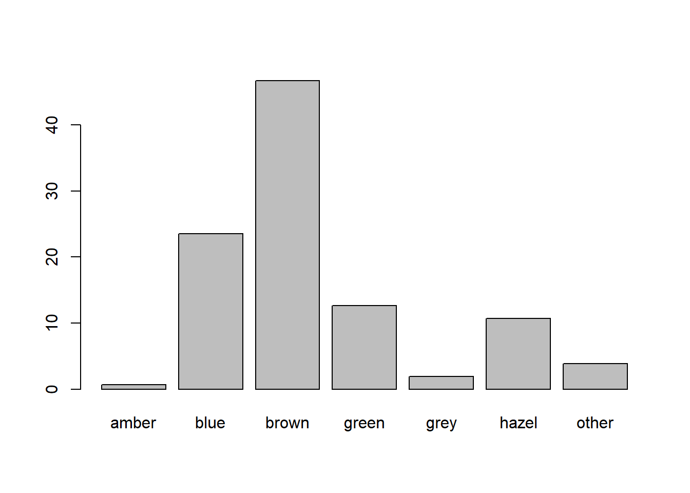
Eye-Colours

Research Question: Do the proportions of people with different eye-colours correspond to those suggested by the internet?

According one part of the internet (that reliable source of information!), 76% of people in the world have brown eyes, 10% have blue, 5% hazel, 5% amber, 2% green, 1% grey, and 1% have some other eye colouring (red/violet/heterochromia).

We’ll use the same data from the course survey’s here:

survey_data <- 
  read_csv("https://uoepsy.github.io/data/surveydata_allcourse22.csv")

Question 7

Perform a \(\chi^2\) goodness of fit test to assess the extent to which our sample of students conform to this theorised distribution of eye-colours.

No need to do this manually - once is enough. Just go straight to using the chisq.test() function.

Hint: Try using chisq.test(..., p = c(?,?,?,...) ).
We saw this in the example goodness of fit test, 4A #example

Solution

Let’s look at the observed counts:

table(survey_data$eyecolour)

amber  blue brown green  grey hazel other 
    3   110   218    59     9    50    18 

Our theoretical probabilities of different eye colours must match the order in the table which we give chisq.test(). They must also always sum to 1.

chisq.test(table(survey_data$eyecolour), p = c(.05,.1,.76,.02,.01,.05,.01))

Warning in chisq.test(table(survey_data$eyecolour), p = c(0.05, 0.1, 0.76, :
Chi-squared approximation may be incorrect

    Chi-squared test for given probabilities

data:  table(survey_data$eyecolour)
X-squared = 492.87, df = 6, p-value < 2.2e-16

Note, we get a warning here of “Chi-squared approximation may be incorrect”. This is because some of the expected cell counts are <5.

chisq.test(table(survey_data$eyecolour), 
           p = c(.05,.1,.76,.02,.01,.05,.01))$expected

 amber   blue  brown  green   grey  hazel  other 
 23.35  46.70 354.92   9.34   4.67  23.35   4.67 

There are a couple of options here, but the easiest is to use the functionality of chisq.test() that allows us to compute the p-value by using a simulation (similar to the idea we saw in 2B#sampling-&-sampling-distributions), rather than by comparing it to a theoretical \(\chi^2\) distribution. We can do this by using:

chisq.test(table(survey_data$eyecolour), p = c(.05,.1,.76,.02,.01,.05,.01),
           simulate.p.value = TRUE)

    Chi-squared test for given probabilities with simulated p-value (based
    on 2000 replicates)

data:  table(survey_data$eyecolour)
X-squared = 492.87, df = NA, p-value = 0.0004998

Question 8

What are the observed proportions of our sample with each eyecolour?
Can you figure out how to use the prop.table() function?

Solution

From the help documentation (?prop.table()), we see that we can pass prop.table() the argument x, which needs to be a table.

prop.table(table(survey_data$eyecolour))*100

     amber       blue      brown      green       grey      hazel      other 
 0.6423983 23.5546039 46.6809422 12.6338330  1.9271949 10.7066381  3.8543897 

barplot(prop.table(table(survey_data$eyecolour))*100)

Jokes and Tips

Data: TipJokes

Research Question: Can telling a joke affect whether or not a waiter in a coffee bar receives a tip from a customer?

A study published in the Journal of Applied Social Psychology¹ investigated this question at a coffee bar of a famous seaside resort on the west Atlantic coast of France. The waiter randomly assigned coffee-ordering customers to one of three groups. When receiving the bill, one group also received a card telling a joke, another group received a card containing an advertisement for a local restaurant, and a third group received no card at all.

The data are available at https://uoepsy.github.io/data/TipJoke.csv.
The dataset contains the variables:

• Card: None, Joke, Ad.
• Tip: 1 = The customer left a tip, 0 = The customer did not leave tip.

Question 9

Produce a plot and a table to display the relationship between whether or not the customer left a tip, and what (if any) card they received alongside the bill.

Don’t worry about making it all pretty. Mosaic plots in R are a bit difficult.

Hint:
plot(table(...)) will give you something. You can see one in the example \(\chi^2\) test of independence,4A #example-1.

Solution

tipjoke <- read_csv('https://uoepsy.github.io/data/TipJoke.csv')

table(tipjoke$Card, tipjoke$Tip)

      
        0  1
  Ad   60 14
  Joke 42 30
  None 49 16

plot(table(tipjoke$Card, tipjoke$Tip))

Question 10

What would you expect the cell counts to look like if there were no relationship between what the waiter left and whether or not the customer tipped?

Solution

In total, 60 customers tipped (14+30+16), and 151 did not. So overall, 0.28 (\(\frac{60}{(60+151)}\)) of customers tip.

74 customers got an Ad card, 72 customers got a Joke, and 65 got None. If this were independent of whether or not they left a tip, we would expect equal proportions of tippers in each group.
So we would expect 0.28 of each group to leave a tip.

You can think about observed vs expected by looking at the two-way table along with the marginal row and column totals given:

	0	1
Ad			74
Joke			72
None			65
	151	60	211

For a given cell of the table we can calculate the expected count as \(\text{row total} \times \frac{\text{column total}}{\text{samplesize}}\):

Expected:

	0	1
Ad	52.96	21.04	74
Joke	51.53	20.47	72
None	46.52	18.48	65
	151.00	60.00	211

If you’re wondering how we do this in R.. here’s our table:

t <- tipjoke %>%
  select(Card, Tip) %>% table()
t

      Tip
Card    0  1
  Ad   60 14
  Joke 42 30
  None 49 16

Here are the row totals:

rowSums(t)

  Ad Joke None 
  74   72   65 

and column totals divided by total:

colSums(t) / sum(t)

        0         1 
0.7156398 0.2843602 

there’s a complicated bit of code using %o% which could do this for us. You don’t need to remember %o%, it’s very rarely used):

e <- rowSums(t) %o% colSums(t) / sum(t)
e

            0        1
Ad   52.95735 21.04265
Joke 51.52607 20.47393
None 46.51659 18.48341

Or, alternatively, do it one by one:

rowSums(t) * (colSums(t) / sum(t))[1]

      Ad     Joke     None 
52.95735 51.52607 46.51659 

rowSums(t) * (colSums(t) / sum(t))[2]

      Ad     Joke     None 
21.04265 20.47393 18.48341 

Question 11

Just like we gave the chisq.test() function a table of observed frequencies when we conducted a goodness of fit test in earlier exercises, we can give it a two-way table of observed frequencies to conduct a test of independence.

Try it now.

Solution

chisq.test(table(tipjoke$Card, tipjoke$Tip))

    Pearson's Chi-squared test

data:  table(tipjoke$Card, tipjoke$Tip)
X-squared = 9.9533, df = 2, p-value = 0.006897

Some RMarkdown

For one of the \(t\)-tests we saw in the previous week’s exercises, we can use an RMarkdown document in which we write our results so that they get compiled to look nice and pretty:

Writing this

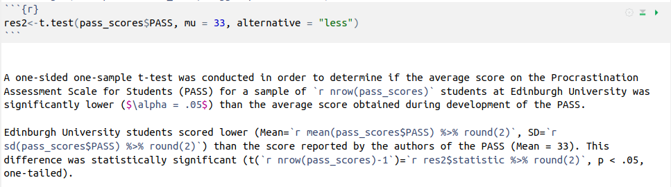
Compiles to this

A one-sided one-sample t-test was conducted in order to determine if the average score on the Procrastination Assessment Scale for Students (PASS) for a sample of 20 students at Edinburgh University was significantly lower (\(\alpha = .05\)) than the average score obtained during development of the PASS.

Edinburgh University students scored lower (Mean = 30.7, SD = 3.31) than the score reported by the authors of the PASS (Mean = 33). This difference was statistically significant (t(19)=-3.11, p < .05, one-tailed).

This is one of the huge benefits of RMarkdown. Imagine we collected more data - we wouldn’t have to edit all the results, we could simply recompile and they would update for us!
Note how it works:

• the code chunk saves the results of the t.test() function as a named object res2.
• in text, the backticks `r … … … ` are used to execute small bits of R code, and include the output within the text. For instance, the line `r res2$statistic %>% round(2)` gets the t-statistic from the results, and rounds it to 2 decimal places, which get’s printed out as -3.11.
• the bits between the dollar signs, e.g. $\alpha$ will get printed as mathematical symbols such as \(\alpha\).

RMarkdown documents are self-contained.

You need to to put everything that is needed to reproduce your analysis in the correct order.

For instance, if you have used the console (bottom left window) to define an object peppapig <- 30, you will have an object in your environment (top right window) called “peppapig” which has the value 30.

If you were to refer to that object in your RMarkdown document, you will be able to run a line of code such as peppapig/10 because it will find the “peppapig” object in your environment. BUT you won’t be able to compile the document because it “starts fresh” (i.e., compiles within its own environment). In order for it to compile, you would need to define what “peppapig” is inside your document, and before the document then refers to it.

The same applies with using functions in from packages. The RMarkdown document needs to know what packages to load before it uses functions from them. Just because you yourself have loaded a package in your session, it does not mean the compilation process for your RMarkdown has access to it.

If you want some extra explanations on these aspects of RMarkdown, then please see Lessons 0-3 of our Rmd-bootcamp.

Question 12

Can you create an RMarkdown document which:

1. Reads in the https://uoepsy.github.io/data/TipJoke.csv data.
2. Conducts and reports a \(\chi^2\) test of independence examining whether telling a joke affect whether or not a waiter in a coffee bar receives a tip from a customer.
3. Successfully compiles (“knits”) into an .html file.

Footnotes

1. Gueaguen, N. (2002). The Effects of a Joke on Tipping When It Is Delivered at the Same Time as the Bill. Journal of Applied Social Psychology, 32(9), 1955-1963.