Week 2 Exercises: More R; Estimates & Intervals

In the last couple of years during welcome week, we have asked students of the statistics courses in the Psychology department to fill out a little survey.
Anonymised data are available at https://uoepsy.github.io/data/surveydata_allcourse22.csv.

Data manipulation & visualisation

Question 1

Create a new variable in the dataset which indicates whether people are taller than 6 foot (182cm).

Hints:
You might want to use mutate(). Remember to make the changes apply to the objects in your environment, rather than just printing it out.
data <- data %>% mutate(...)
(see 2A #tidyverse-and-pipes)

Solution

library(tidyverse)
surveydata <- read_csv("https://uoepsy.github.io/data/surveydata_allcourse22.csv")

surveydata <- surveydata %>%
  mutate(
    over6ft = height > 182
  )

Question 2

What percentage of respondents to the survey (for whom we have data on their height) are greater than 6 foot tall?

Hints:

• Try table(), and then think about how we can convert the counts to percentages (what does sum() of the table give you?).
  • table() will actually by default count only those values which aren’t missing, so this means you don’t have to do anything extra here (if you wanted it to also count the missing values, we can use table(data$variable, useNA = "ifany"))
• See also 2A #categorical.

Solution

We can divide the table by the sum of the table

table(surveydata$over6ft) / sum(table(surveydata$over6ft))

     FALSE       TRUE 
0.95670996 0.04329004 

We can also use prop.table()

prop.table(table(surveydata$over6ft))

     FALSE       TRUE 
0.95670996 0.04329004 

Question 3

how many of USMR students in 2022/23 are born in the same month as you?

Hints:
This will involve filtering your data to current USMR students first.
In tidyverse you can make a table using ... %>% select(variable) %>% table()
You can also try ... %>% count(variable) to get the same information.

Solution

surveydata %>% 
  filter(course == "usmr", year=="2022") %>%
  count(birthmonth)

# A tibble: 12 × 2
   birthmonth     n
   <chr>      <int>
 1 apr            7
 2 aug            6
 3 dec            6
 4 feb            1
 5 jan            4
 6 jul           12
 7 jun           10
 8 mar            6
 9 may           10
10 nov            7
11 oct            4
12 sep            5

Question 4

Calculate the mean and standard deviation of heights of all respondents to the survey.

Can you (also) do this using the tidyverse syntax?

Hints:
We can do it with mean(data$variable), but it will be useful to practice tidyverse style. You’ll want to summarise() the data.
We’re likely to have missing data in here, so na.rm=TRUE will be handy (see 2A #numeric)

Solution

This returns us NA:

mean(surveydata$height)

[1] NA

So we need to make sure we use na.rm = TRUE (we can use T as a shorthand for TRUE).

mean(surveydata$height, na.rm = T)

[1] 167.8975

sd(surveydata$height, na.rm = T)

[1] 8.369403

surveydata %>% 
  summarise(
    meanheight = mean(height, na.rm = T),
    sdheight = sd(height, na.rm = T)
  )

# A tibble: 1 × 2
  meanheight sdheight
       <dbl>    <dbl>
1       168.     8.37

Question 5

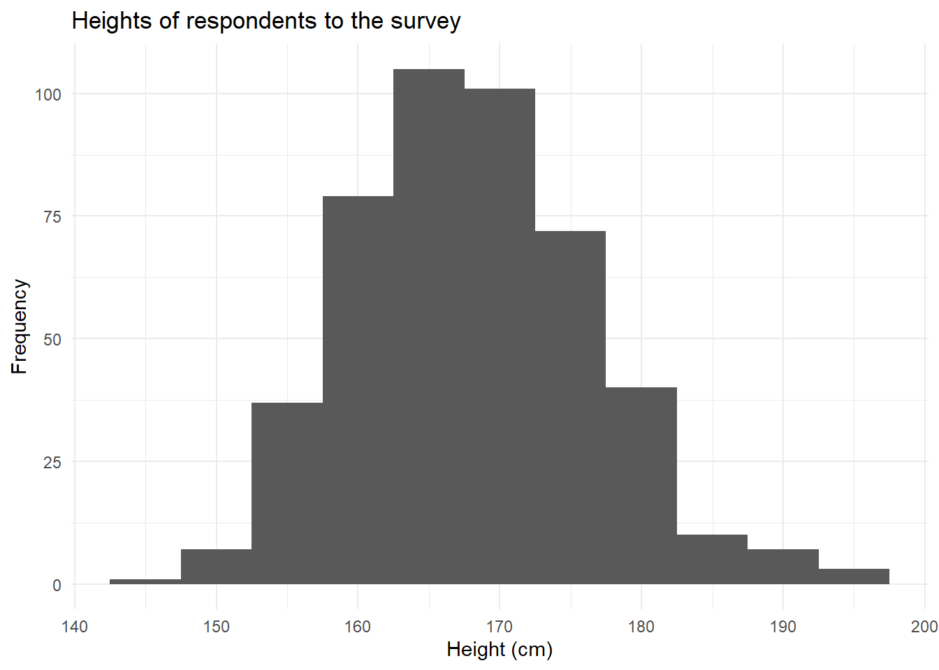
Plot the distribution of heights of all respondents. Try to make it ‘publication ready’.

Hints:
hist() won’t cut it here, we’re going to want ggplot, which was introduced in 2A #ggplot.

Solution

ggplot(surveydata, aes(x=height)) + 
  geom_histogram(binwidth = 5) + 
  labs(x = "Height (cm)", 
       y = "Frequency", 
       title = "Heights of respondents to the survey") + 
  theme_minimal()

Question 6

For respondents from each of the different courses, calculate the mean and standard deviation of heights.

Hints:
This is just like question 4 - we want to summarise our data. Only this time we need to group_by something else first.

Solution

We’re using the same code as we did for question 4, but we’ve added in one new line using group_by().

surveydata %>% 
  group_by(course) %>%
  summarise(
    meanheight = mean(height, na.rm = T),
    sdheight = sd(height, na.rm = T)
  )

# A tibble: 4 × 3
  course meanheight sdheight
  <chr>       <dbl>    <dbl>
1 dapr1        168.     7.36
2 dapr2        167.     7.79
3 rms2         167.     7.98
4 usmr         168.     9.08

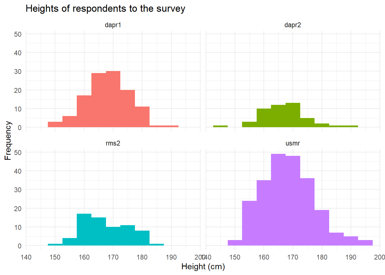
Question 7

Plot the distributions of heights for each course.
Based on your answer to the previous question, can you picture what the distributions are going to look like before you plot them?

Hints:
Try looking up the documentation for ?facet_wrap. It is an incredibly useful extension of ggplot which allows you to create the same plot for different groups.

You might also want to add an extra aesthetic mapping from the course variable to some feature of your plot (e.g. ‘colour’ or ‘fill’).

Solution

ggplot(surveydata, aes(x=height, fill = course)) + 
  geom_histogram(binwidth = 5) + 
  facet_wrap(~course) + 
  labs(x = "Height (cm)", 
       y = "Frequency", 
       title = "Heights of respondents to the survey") + 
  guides(fill = "none") + 
  theme_minimal()

Question 8

What proportion of respondents to the survey are taller than you?

Hints:

• Remember that we can sum() a condition as a quick way of counting: sum(data$variable == "thing") adds up all the TRUE responses.
  • We’re going to need to make sure we tell sum() to ignore the missing values (na.rm=TRUE will come in handy again).
    
• We’re also going to need to figure out what our denominator is when calculating the proportion \(\frac{\text{nr people taller than me}}{\text{total nr of people}}\).
  The denominator (the bit on the bottom) should really be the total number of people for whom we have height data. We should exclude the missing data because otherwise we will be counting them as if they are all shorter than you (but they might not be - we don’t know!). To find out how many in a variable are not NAs, we might need to use is.na() (see below for a little example for you to play with)
• Can you also do this in tidyverse syntax? (most of it can be done inside summarise()).

is.na()

The is.na(x) function is a bit like asking x == NA. It is necessary because NA is a special thing in R, which means we can’t ask questions like 3 == NA (because we don’t know what that NA is - it could be 3 for all we know!).

mynumbers <- c(1,5,NA,3,6,NA)
# for each number, TRUE if it's an NA, otherwise FALSE
is.na(mynumbers)

[1] FALSE FALSE  TRUE FALSE FALSE  TRUE

# ! means "not", so this is asking if each number is "not" an NA
!is.na(mynumbers)

[1]  TRUE  TRUE FALSE  TRUE  TRUE FALSE

# how many non-NAs are there? 
sum(!is.na(mynumbers))

[1] 4

Solution

There are this many people who are taller than me. We need to ignore the NAs again:

sum(surveydata$height > 177, na.rm = T)

[1] 60

To get the total number of respondents with height data, we can sum the non-NA values:

sum(!is.na(surveydata$height))

[1] 462

And if we divide the number who are taller than me by the total number of respondents, we get the proportion:

sum(surveydata$height > 177, na.rm = T) / sum(!is.na(surveydata$height))

[1] 0.1298701

We can do all this inside tidyverse too!

surveydata %>% 
  summarise(
    n_taller = sum(height > 177, na.rm = T),
    n_heights = sum(!is.na(height)),
    prop_taller = n_taller / n_heights
  )

# A tibble: 1 × 3
  n_taller n_heights prop_taller
     <int>     <int>       <dbl>
1       60       462       0.130

Estimates & Intervals

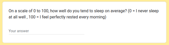
For these next exercises we are going to be focusing on self-perceived sleep quality ratings. Our survey contains a set of respondents who completed the question below. We’re going to use this sample to get an estimate of the sleep quality rating in the wider population.

Question 9

We only asked the sleep quality rating question to students in USMR in the 2022/23 academic year, so to make things easier, let’s create a subset of the dataset which includes only those students.

Hints:
This will need some filtering, and assigning (usmrdata <-) to a new name.

Solution

usmrdata <- surveydata %>% 
  filter(course == "usmr", year == "2022")
dim(usmrdata)

[1] 78 21

Question 10

For the USMR students in the 2022/23 academic cohort, calculate the following:

• mean Sleep-Quality rating
• standard deviation of Sleep-Quality ratings
• number of respondents who completed Sleep-Quality rating

Hints:
You can do this with things like mean(data$variable), or you can do it all in tidyverse (see the example of summarise in the intro to tidyverse: 2A #tidyverse-and-pipes).

Solution

usmrdata %>% 
  summarise(
    m_sleep = mean(sleeprating, na.rm = TRUE),
    sd_sleep = sd(sleeprating, na.rm = TRUE),
    n_sleep = sum(!is.na(sleeprating)), 
    n_total = n() # n() will give the total count
  )

# A tibble: 1 × 4
  m_sleep sd_sleep n_sleep n_total
    <dbl>    <dbl>   <int>   <int>
1    65.5     22.7      77      78

Question 11

Using your answers to the previous question, construct a 95% confidence interval for the average Sleep-Quality rating.

Why might it be a bad idea to use this as an estimate of the average Sleep-Quality rating of the global population?

Hints:

• The previous question gives you all the pieces that you need. You’ll just need to put them together in the way seen in 2B #confidence-intervals.
  
• Think about who makes up the sample (e.g. USMR students). Are they representative of the population we are trying to generalise to?

Solution

So we have our estimate, which is the mean sleep quality rating in our sample: \(\bar x = 65.51\). And we have a standard deviation of our sleep quality ratings: \(s = 22.7\). While our sample has 78 students in it, only 77 responded to the sleep question, so really our \(n\) for this calculation is 77.

We can calculate our standard error as \(SE = \frac{s}{\sqrt{n}}\), which is \(\frac{22.7}{\sqrt{77}} = 2.59\).

This tells us that if we were to collect lots of samples of size 77, we would expect their mean sleep quality ratings to be normally distributed around 65.51 with a standard deviation of 2.59. So we can expect that 95% of the samples we could take would have means between \(1.96 \times 2.59\) above and below 65.51. Those are our confidence intervals!

\[ \begin{align} \text{Mean = }& 65.51 \\ \text{95\% CI = }& 65.51 \pm 1.96 \times 2.59 \\ &[60.43, 70.59] \end{align} \]

How well does our sample represent the global population? Well, for one thing, you’re all university students, and while there will be many students from across the globe, it’s highly likely that our sample is biased towards certain countries or continents. Additionally, we’re going to have a lot of people in our sample in a fairly narrow age range. It might be that sleep quality changes a lot as people age, in which case our results are probably not going to generalise very well to, for instance, people who are 70 years old. There are lots more ways in which our sample might be biased - you can find a nice little 1 page article at https://www.nature.com/articles/466029a to get you thinking.

`