Week 10 Exercises: Logistic Regression

Odd Probability

Question 1
  1. The probability of a coin landing on heads if 0.5, or 50%. What are the odds, and what are the log-odds?
  2. Last year’s Tour de France winner, Tadej Pogacar, was given odds of 11 to 4 by a popular gambling site (i.e., if we could run the race over and over again, for every 4 he won he would lose 11). Translate this into the implied probability of him winning.

Hints:

  1. A 50% chance of landing on heads is equivalent to the odds of \(\frac{0.5}{(1-0.5)} = \frac{0.5}{0.5} = \frac{1}{1}\) (odds of 1 to 1, i.e., “equal odds”).
    The log-odds can be calculated using log(1) in R, which returns 0.

  2. If Pogacar is predicted to win 4 for every 11 he loses, then this is means he is predicted to win 4 in every 15 races, so the implied probability of him winning is \(\frac{4}{15} = 0.267\).

Drunkdoor

Research Questions Is susceptibility to change blindness influenced by level of alcohol intoxication and perceptual load?

Method Researchers conducted a study in which they approached 120 people, recruited from within the vicinity of a number of establishments with licenses to sell alcohol to be consumed on-premises. Initially, experimenter A approached participants and asked if they were interested in participating in a short study, and obtained their written consent. While experimenter A subsequently talked each participant through a set of questions on multiple pieces of paper (with the pretense of explaining what the participant was required to do), experimenters B and C carrying a door passed between the participant and experimenter A, with experimenter C replacing A (as can be viewed in the video below).

Simons, D. J., & Levin, D. T. (1997). Change blindness. Trends in cognitive sciences, 1(7), 261-267.

The perceptual load of the experiment was manipulated via a) the presentation of the door and b) the papers held by the experimenters. For 60 of these participants, the door was painted with some detailed graffiti and had a variety of pieces of paper and notices attached to the side facing the participants. Additionally, for these participants, the experimenters handled a disorganised pile of 30 papers, with the top pages covered in drawings around the printed text. For the remaining 60, the door was a standard MDF construction painted a neutral grey, and the experimenters handled only 2 sheets of paper which had minimal printed text on them and nothing else.

Measures
After experimenters A and C had successfully swapped positions, the participant was asked (now by C) to complete small number of questions taking approximately 1 minute. Either after this set of questions, or if the participant made an indication that they had noticed the swap, the experimenters regrouped and the participant was explicitly asked whether they had noticed the swap.
Immediately after this, participants were breathalysed, and their blood alcohol content was recorded. In addition, participants’ age was recorded, as previous research suggests that change-blindness increases with age.

Data

The data can be downloaded from https://uoepsy.github.io/data/drunkdoor.csv.
A description of the variables included is presented below.

variable description
id Unique ID number
bac Blood Alcohol Content (BAC), A BAC of 0.0 is sober, while in the United States 0.08 is legally intoxicated, and above that is very impaired. BAC levels above 0.40 are potentially fatal.
age Age (in years)
condition Condition - Perceptual load created by distracting oject (door) and details and amount of papers handled in front of participant (Low vs High)
notice Whether or not the participant noticed the swap (Yes = 1 vs No = 0)

Age effects

Question 2

To begin with, we’re going to ignore the research question, and just look at the relationship between age and whether or not participants noticed the person-switch.

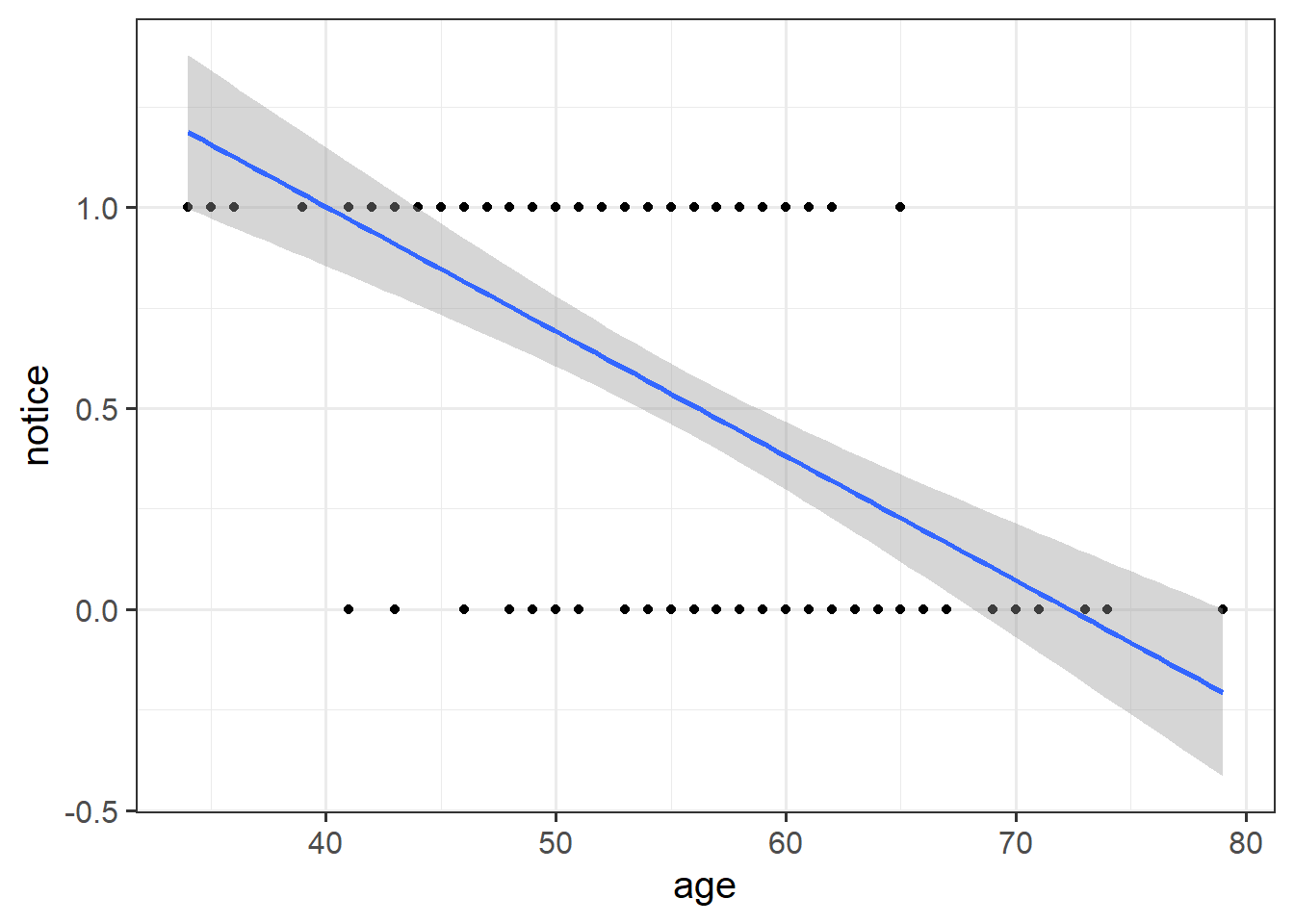
Make a scatterplot of this relationship, and add to the plot geom_smooth(method="lm"). This will plot the regression line for a simple model of lm(notice ~ age).

Hint: It won’t look very nice!

drunkdoor <- read_csv("https://uoepsy.github.io/data/drunkdoor.csv")

ggplot(drunkdoor, aes(x=age, y=notice))+
  geom_point()+
  geom_smooth(method="lm")

Question 3

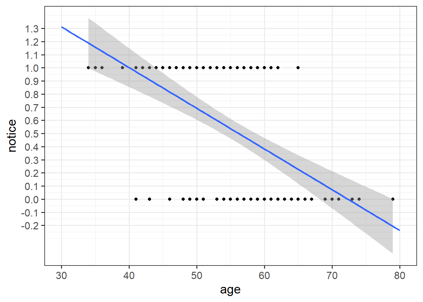
Just visually following the line from the plot produced in the previous question, what do you think the predicted model value would be for someone who is aged 30?
What does this value mean?

Hint: There’s not really an answer to this.

This plot will make it easier to see that the model predicted value for someone aged 30 is approximately 1.15.

What does 1.15 really mean here? A 30 year old participant will notice 1.15 experimenter-swaps? They have a 115% probability of noticing the swap? That is maybe closer, but we can’t have such a probability - probability is between 0 and 1.

Question 4

Fit a logistic regression model investigating whether participants’ age predicts the log-odds of noticing the person they are talking to being switched out mid-conversation. Look at the summary() output of your model.

Hints:

  • To fit a logistic regression model, we need to useglm(), a slightly more general form of lm().
  • The syntax is pretty much the same, but we need to add in a family at the end, to tell it that we are doing a binomial1 logistic regression.
  • See 10A#fitting-glm-in-r

model1 <- glm(notice ~ age, data = drunkdoor, family=binomial(link="logit"))
summary(model1)

Call:
glm(formula = notice ~ age, family = binomial(link = "logit"), 
    data = drunkdoor)

Coefficients:
            Estimate Std. Error z value Pr(>|z|)    
(Intercept)  10.2270     1.9634   5.209 1.90e-07 ***
age          -0.1819     0.0349  -5.213 1.86e-07 ***
---
Signif. codes:  0 '***' 0.001 '**' 0.01 '*' 0.05 '.' 0.1 ' ' 1

(Dispersion parameter for binomial family taken to be 1)

    Null deviance: 166.06  on 119  degrees of freedom
Residual deviance: 120.28  on 118  degrees of freedom
AIC: 124.28

Number of Fisher Scoring iterations: 5

Question 5

Based on your model output, complete the following sentence:

“Being 1 year older decreases _________ by 0.18.”

Hint: on what scale (probability, odds, log-odds) are we modelling linear associations?

“Being 1 year older decreases the log-odds of noticing a mid-conversation person switch by 0.18.”

Question 6

To get this association into something that is (slightly) more easy to understand, exponentiate the coefficients from your model in order to translate them back from log-odds in to “odds ratios”. Provide an interpretation of what the resulting estimates mean.

Hints:

exp(coef(model1))
 (Intercept)          age 
2.763972e+04 8.336732e-01 
  • The odds of noticing a mid-conversation person-switch for someone age 0 is 27639:1.
  • For every year older someone is, the odds of noticing the switch are multiplied by 0.83.

Question 7

Based on your answer to the previous question, calculate the odds of noticing the swap for a one year-old (for now, forget about the fact that this experiment wouldn’t work on a 1 year old!)
And what about for a 40 year old?

Can you translate the odds back in to probabilities?

exp(coef(model1))
 (Intercept)          age 
2.763972e+04 8.336732e-01 

The odds of noticing a mid-conversation person-switch for someone age 0 is 27639:1.
For every year older someone is, the odds of noticing decrease by 0.83.

For a one year old

This means that for a one year old, the odds of noticing are \(27640 \times 0.83\), or more precisely \(27640 \times 0.8336732\):

exp(coef(model1)[1]) * exp(coef(model1)[2])
(Intercept) 
   23042.49 

So the odds for a one-year old are 23042:1.

We can also get to this using addition on the log-odds scale:

coef(model1)[1] + coef(model1)[2]
(Intercept) 
    10.0451 

and then exponentiating it:

exp(10.0451)
[1] 23042.6

For a 40 year old

The odds for a 40 year old are \(27640 \times 0.83 \times 0.83 \times 0.83 \times 0.83 \times 0.83 \times ...\) or \(27640 \times 0.83^{40}\).

exp(coef(model1)[1]) * exp(coef(model1)[2])^40
(Intercept) 
   19.11465 

Or using log-odds:

( coef(model1)[1] + (coef(model1)[2]*40) ) %>% 
  exp()
(Intercept) 
   19.11465 

Converting to probabilities

And we can now turn these back into probabilities.

Predicted probability of noticing for a one year old = \(\frac{23042.6}{1 + 23042.6} = 0.9999\) Predicted probability of noticing for a 40 year old = \(\frac{19.11}{1 + 19.11} = 0.95\)

Question 8

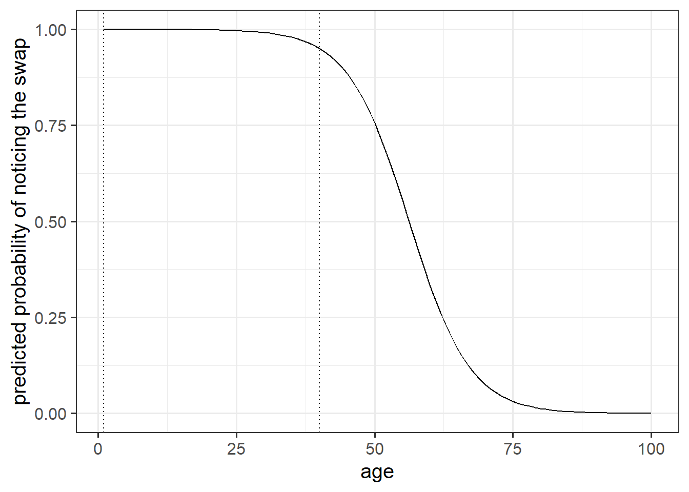
It’s possible to calculate predicted probabilities for a specific value of the predictor(s), but what would be nice is to see how the probability of noticing the swap changes with age.

The code below creates a dataframe with the variable age in it, which has the values 1 to 100. Can you use this object and the predict() function, along with your model, to calculate the predicted probabilities of the outcome (noticing the swap) for each year of age from 1 to 100?
Can you then plot this?

ages100 <- tibble(age = 1:100)

Hints:

  • predict(model, newdata = ???)
  • try seeing what happens to the plot when you change between:
    • predict(model, newdata = ???, type = "link")
    • predict(model, newdata = ???, type = "response")
  • 10A#visualising

This will spit out the predicted probabilities for each observation

predict(model1, newdata = ages100, type = "response")

Let’s add them to the ages100 tibble

ages100 <- 
  ages100 %>%
  mutate(
    predprobs = predict(model1, newdata = ages100, type = "response"),
    predlogodds = predict(model1, newdata = ages100, type = "link")
  )

and plot them against age! We can also add those two people (the 1 year old and the 40 year old) that we were predicting in the earlier question

ggplot(data = ages100, aes(x = age, y = predprobs)) +
  geom_line()+
  labs(y="predicted probability of noticing the swap")+
  geom_vline(xintercept=c(1,40), lty="dotted")

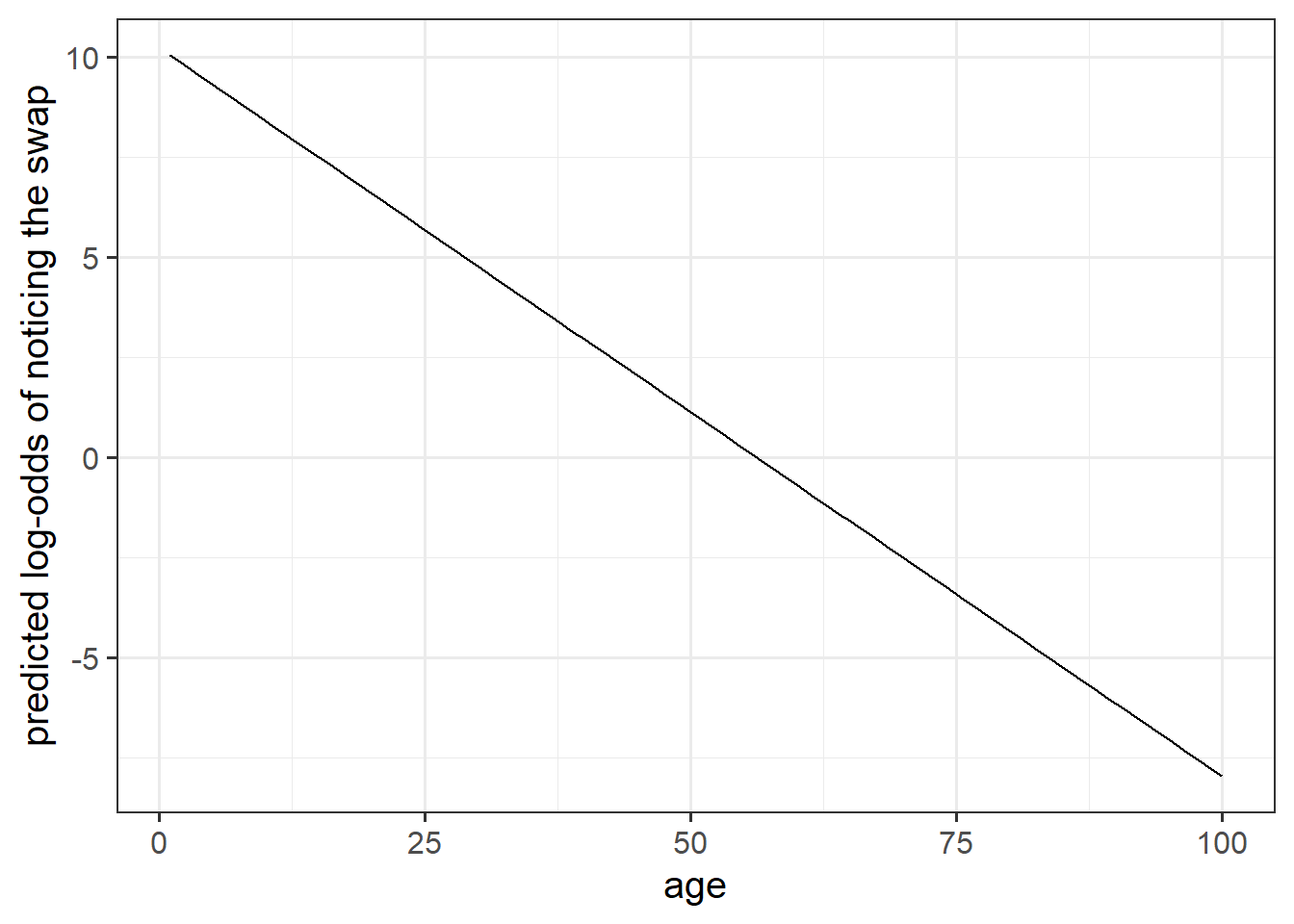
Note that the predict(model, type="link") gives us the estimated log-odds. If we plot those:

ggplot(data = ages100, aes(x = age, y = predlogodds)) +
  geom_line()+
  labs(y="predicted log-odds of noticing the swap")

Tackling the research question

Question 9

Recall our research question, which we will now turn to:

Research Questions Is susceptibility to change blindness influenced by level of alcohol intoxication and perceptual load?

Try and make a mental list of the different relationships between variables that this question invokes, can you identify one variable as the ‘outcome’ or ‘response’ variable? (it often helps to think about the implicit direction of the relationship in the question)

In addition, are there known things that it might be useful to account for, so that you capture associations that are independent from differences due to these things (hint hint, what have you just been looking at?).

The question seems to ask about two relationships:

  • susceptibility to change blindness ← alcohol intoxication
  • susceptibility to change blindness ← perceptual load

and we know (from previous research, as well as our previous exercises) that change-blindness is associated with age.

The arrows above are used to show the implied direction of the influence, and in the lm()/glm() syntax, you could imagine each of these mapping to a formula syntax we have seen a few times (e.g., t.test(outcome ~ group) and lm(outcome ~ predictor)). We can see that the ‘susceptibility to change blindness’ is our outcome variable:

  • change blindness ~ alcohol
  • change blindness ~ perceptual load
  • and we also have reason to think change blindness ~ age

As a general rule of thumb, it is often worth asking yourself “why run multiple models when one will do?”. Think about what we have learned about moving from simple to multiple regression - some of the explanatory power of x in the relationship y~x might be shared by the relationship y~z.
This will depend on precisely what quantity you want to estimate, i.e., “the overall effect of \(x\) on \(y\) ignoring \(z\)” or “the effect of \(x\) on \(y\) after accounting for differences due to \(y\)”. The former statement might indicate a simple bivariate relationship, and the latter requires more advanced techniques (e.g., multiple regression).

Question 10

Think about our outcome variable and how it is measured. What type of data is it? Numeric? Categorical?

What type of distribution does it follow? For instance, do values vary around a central point, or fall into one of various categories, or follow the count of successes in a number of trials?

Our outcome variable here is drunkdoor$notice, and is stored as a set of 0s and 1s. These are the only two values that an observation can take, and they represent the number of successes in n = 1 trial.

So, from this we learn that our method of analysis should be suited to model this binary outcome. So things like lm() and t.test() are not very suitable.

Question 11

Think about our explanatory variable(s). Is there more than one? What type of variables are they? Do we want to model these together? Might they be correlated?

Solution

Question 12
  1. Write a sentence describing the model you will fit. It might help to also describe each variable as you introduce it.
  2. Fit the model.

Hints:

Think of this as writing out the R code but in words.
For instance: glm(outcome ~ predictor1 + predictor2 + Predictor1:Predictor2, family = binomial) might be described as “Outcome (binary,”Level 1” vs “Level 2”) was modelled using logistic regression, predicted by Predictor1, Predictor2 and their interaction”

  • Do you want BAC on the current scale, or could you transform it somehow?
  • Is condition a factor? What is your reference level? Have you checked contrasts(drunkdoor$condition)? (Remember that this will only work if you make it a factor first)

Whether or not participants noticed the swap mid-conversation (binary 0 vs 1) is modelled using logistic regression, with blood alcohol content (measured in 100th of percentages blood content) and perceptual load condition (low load vs high load, with low as the reference level) and age (in years, mean centered).

In the sentence above, I stated that I want blood alcohol in terms of 100ths of percentages, rather than percentages. And I want age centered on the mean (this won’t change anything other than the intercept).

drunkdoor <- drunkdoor %>% 
  mutate(
    bac100 = bac*100,
    ageC = age - mean(age)
  )

I also stated that the low-load will be the reference level.
Currently it will be the other way around, because “high” comes before “low” in the alphabet. I can change it:

# make it a factor and give it the levels in the right order
# note this requires getting the levels named exactly as they appear in the variable. 
# if we use lowercase "low", then every "Low" in the variable will turn to NA
drunkdoor$condition <- factor(drunkdoor$condition, levels = c("Low","High"))
# check the contrasts
contrasts(drunkdoor$condition)
     High
Low     0
High    1

Finally, let’s fit our model!

changeblind_model <- glm(notice ~ ageC + bac100 + condition, data = drunkdoor, family = "binomial")
summary(changeblind_model)

Call:
glm(formula = notice ~ ageC + bac100 + condition, family = "binomial", 
    data = drunkdoor)

Coefficients:
              Estimate Std. Error z value Pr(>|z|)    
(Intercept)   -0.51577    0.53536  -0.963  0.33534    
ageC          -0.22584    0.04214  -5.359 8.35e-08 ***
bac100         0.35002    0.11128   3.145  0.00166 ** 
conditionHigh -1.59215    0.54008  -2.948  0.00320 ** 
---
Signif. codes:  0 '***' 0.001 '**' 0.01 '*' 0.05 '.' 0.1 ' ' 1

(Dispersion parameter for binomial family taken to be 1)

    Null deviance: 166.06  on 119  degrees of freedom
Residual deviance: 100.99  on 116  degrees of freedom
AIC: 108.99

Number of Fisher Scoring iterations: 5

Question 13

Compute 95% confidence intervals for the log-odds coefficients using confint(). Wrap the whole thing in exp() in order to convert all these back into odds and odds-ratios.

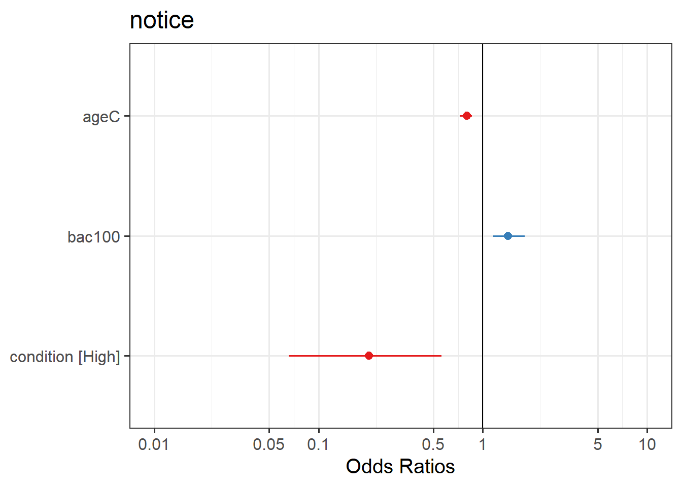
Try the sjPlot package and using tab_model(model) and plot_model(model, type = "est") on your model. What do you get?

confint(changeblind_model)
                   2.5 %     97.5 %
(Intercept)   -1.5931147  0.5259275
ageC          -0.3183866 -0.1514958
bac100         0.1438639  0.5849749
conditionHigh -2.7166875 -0.5805803
exp(confint(changeblind_model))
                   2.5 %    97.5 %
(Intercept)   0.20329144 1.6920275
ageC          0.72732154 0.8594215
bac100        1.15472697 1.7949460
conditionHigh 0.06609332 0.5595736

We can get out the same but in a nice little html table:

library(sjPlot)
tab_model(changeblind_model)
  notice
Predictors Odds Ratios CI p
(Intercept) 0.60 0.20 – 1.69 0.335
ageC 0.80 0.73 – 0.86 <0.001
bac100 1.42 1.15 – 1.79 0.002
condition [High] 0.20 0.07 – 0.56 0.003
Observations 120
R2 Tjur 0.475

And the plot_model with type = "est" gives a nice little way of visualising these odds ratios and confidence intervals.

plot_model(changeblind_model, type = "est") +
  geom_hline(yintercept=1)

Question 14

Write up the results of the study.

Hints:

  • Often when reporting odds ratios, it’s easiest to interpret them as simply “increased odds of (OR = <??> [95% CI: , ])”. This saves a bit of hassle too! &#128516

Whether or not participants noticed the swap mid-conversation (binary 0 vs 1) is modelled using logistic regression, with blood alcohol content (measured in 100th of percentages blood content) and perceptual load condition (low load vs high load, with low as the reference level) and age (in years, mean centered).

In keeping with previous research, age was associated with susceptibility to change-blindness, as indicated by a decreased odds of noting the mid-conversation swap (\(OR = 0.8,\,\, 95\%\, CI\, [0.73, 0.86]\)), after accounting for differences in blood alcohol levels and perceptual load. In contrary to what might be expected, change-blindness appeared to decrease with alcohol intoxication, with the odds of noticing the swap increasing 1.42 times (\([1.15, 1.79]\)) for every 1/100th of a percentage increase in blood alcohol content, holding age and perceptual load constant. After accounting for age and blood alcohol levels, the odds of noticing the swap were significantly different depending upon the perceptual load, with higher perceptual load associated with 0.2 (\([0.07, 0.56]\)) times the odds of noticing the change.

Results corroborate previous findings of age increasing the susceptibility to changeblindness. Increased perceptual load was also found to increase the chances of people being blind to change, in keeping with the intuition that we have a finite capacity for attention, which is taken up more by more distracting objects. Surprisingly, levels of alcohol intoxication appeared to be associated with a greater chance of noticing change. Further work could investigate possible explanations for this association.

Dog people/Cat people

USMR 2022 Data

The data from the USMR 2022 survey (now closed) can be found at https://uoepsy.github.io/data/usmr2022.csv.

note, this is the survey data just from USMR this year, not other students on other courses or in previous years

Question 15

People often talk about personality differences between “cat people” and “dog people” (e.g. if you’re more introverted then you’re more likely to be a cat person).
In our survey, we forced you to choose between “cat” and “dog”, and we also measured a bunch of personality traits from a set of 50 questions (these were aggregated up into scores for ‘extraversion’, ‘conscientiousness’, and so on).

Fit a model that tries to predict whether someone is a cat- or dog- person, based on aspects of their personality.

Hints:

  • your outcome variable is currently not 0 and 1, but “cat” and “dog”. Remember how R prefers to think of categories - as factors.

usmr <- read_csv("https://uoepsy.github.io/data/usmr2022.csv")

make the outcome a factor

usmr$catdog <- factor(usmr$catdog)

we can see from the ordering of the levels that it will treat “cat” as 0 and “dog” as 1, so our model with glm(catdog ~ ...) will be predicted the logodds of being a dog person:

levels(usmr$catdog)
[1] "cat" "dog"

And we are interested in predicted dog-person-ness vs cat-person-ness by different personality traits:

catdogmod <- glm(catdog ~ extraversion + agreeableness + 
                   conscientiousness + emot_stability + 
                   imagination, 
                 data=usmr, family=binomial)

summary(catdogmod)

Call:
glm(formula = catdog ~ extraversion + agreeableness + conscientiousness + 
    emot_stability + imagination, family = binomial, data = usmr)

Coefficients:
                  Estimate Std. Error z value Pr(>|z|)
(Intercept)       -3.50586    2.48706  -1.410    0.159
extraversion       0.01161    0.03221   0.360    0.719
agreeableness      0.05005    0.04472   1.119    0.263
conscientiousness  0.06285    0.04196   1.498    0.134
emot_stability     0.03074    0.02788   1.102    0.270
imagination       -0.04470    0.03748  -1.193    0.233

(Dispersion parameter for binomial family taken to be 1)

    Null deviance: 108.90  on 78  degrees of freedom
Residual deviance: 102.33  on 73  degrees of freedom
  (1 observation deleted due to missingness)
AIC: 114.33

Number of Fisher Scoring iterations: 4

Using GLM to classify

A table of predicted outcome vs observed outcome sometimes gets referred to as a confusion matrix, and we can think of the different cells in general terms (Figure 1).
Another way to think about how our model is fitted is that it aims to maximise (TP + TN)/n, or, put another way, to minimise (FP+FN)/n. Which is equivalent to the good old idea of minimising sums of squares (where we minimise the extend to which the predicted values differ from the observed values).
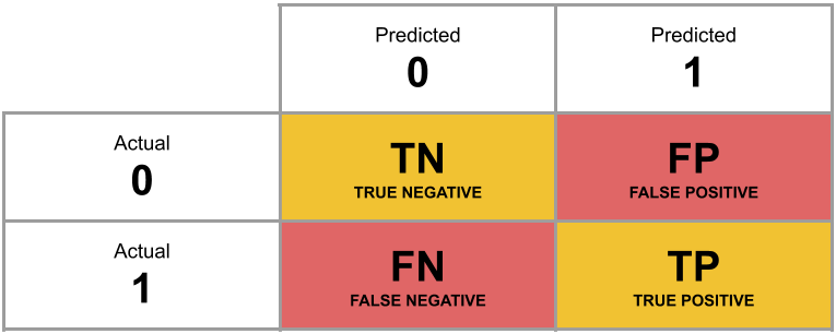
Figure 1: Confusion Matrix
Question 16
  1. Add new column to the survey dataset which contains the predicted probability of being a cat/dog person for each observation.
  2. Then, using ifelse(), add another column which is these predicted probabilities translated into the predicted binary outcome (0 or 1) based on whether the probability is greater than >.5.
  3. Create a two-way contingency table of the predicted outcome and the observed outcome.
  4. What proportion of observations are correctly predicted?

Hint:

  • you don’t need the newdata argument for predict() if you want to use the original data the model was fitted on.
  • if there are NAs in any of the variables in your model (predictors or outcome), then the number of rows in your data will be greater than the number of model predictions.
    • if you want a handy function which might help with this, check out what the broom package has to offer. What does augment(model, type.predict = "response") do?

if we just try to add the predictions to the data, we get an error:

usmr %>%
  mutate(
    predprobs = predict(catdogmod)
  )
Error in `mutate()`:
ℹ In argument: `predprobs = predict(catdogmod)`.
Caused by error:
! `predprobs` must be size 80 or 1, not 79.

We could try making our dataset “complete cases” (remove all rows with any missingness), and then refit our model, and then the data and the model would all be the same number of observations.

However, the broom package has a really useful function which will bring us back the data that was fed into the model (i.e. excluding the NAs), and lots of information about the model fit itself such as predictions (.fitted column), residuals, and leverage etc.

library(broom)
augment(catdogmod, type.predict = "response")
# A tibble: 79 × 13
   .rownames catdog extraversion agreeableness conscientiousness emot_stability
   <chr>     <fct>         <dbl>         <dbl>             <dbl>          <dbl>
 1 1         dog              30            42                33             30
 2 2         dog              34            39                36             31
 3 3         cat              22            44                29             27
 4 4         cat              23            40                35             20
 5 5         dog              16            36                31             27
 6 6         dog              34            44                42             37
 7 7         cat              32            43                32             24
 8 8         dog              32            35                43             16
 9 9         cat              31            42                42             20
10 10        cat              31            43                39             36
# ℹ 69 more rows
# ℹ 7 more variables: imagination <dbl>, .fitted <dbl>, .resid <dbl>,
#   .hat <dbl>, .sigma <dbl>, .cooksd <dbl>, .std.resid <dbl>

So we can use this to get out the observed and the predicted!

augment(catdogmod, type.predict = "response") %>%
  mutate(
    prediction = ifelse(.fitted >.5, "pred_dog", "pred_cat")
  ) %>%
  select(catdog, prediction) %>%
  table() %>% prop.table
      prediction
catdog  pred_cat  pred_dog
   cat 0.2405063 0.2151899
   dog 0.1392405 0.4050633

So 19 cat people are predicted as cat people, and 32 dog people are predicted as dog people. But 17 cat people are predicted as dog-people, and 11 dog people are predicted to be cat people.

\[ \frac{19+32}{19+32+17+11} = \frac{51}{79} = 0.65 \]

65% of observations are correctly predicted by our model.

Optional Extra: Red and White

Question 16

People are a lot more difficult to predict than something like, say, the colour of different wines.

You can download a dataset of 6497 different wines (1599 red, 4898 white) from https://uoepsy.github.io/data/usmr_wines.csv.

It contains information on various physiochemical properties such as pH, a measure of level of sulphates, residual sugar, citric acid, volatile acidity and alcohol content, and also quality ratings from a sommelier (wine expert). All the wines are vinho verde from Portugal, and the data was collected between 2004 and 2007.

Build a model that predicts the colour of wine based on all available information.
How accurately can it predict wine colours?

Hints:

  • glm(outcome ~ ., data = mydata) is a shorthand way of putting all variables in the data in as predictors.
  • Generally speaking, this question doesn’t reflect how we do research in psychology. Ideally, we would have a theoretical question that motivates the inclusion (and testing of) specific predictors.

wines <- read_csv("https://uoepsy.github.io/data/usmr_wines.csv")

wines$col <- factor(wines$col)

winemod <- glm(col ~ ., data = wines, family = binomial)

broom::augment(winemod, type.predict="response") %>%
  mutate(
    pred = ifelse(.fitted>.5,"white","red")
  ) %>%
  select(col,pred) %>% 
  table() %>% 
  prop.table()
       pred
col            red      white
  red   0.20917346 0.03694013
  white 0.02616592 0.72772049
broom::augment(winemod, type.predict="response") %>%
  mutate(
    pred = ifelse(.fitted>.5,"white","red"),
    correct = ifelse(pred==col, 1, 0)
  ) %>%
  select(correct) %>%
  table() %>%
  prop.table()
correct
         0          1 
0.06310605 0.93689395 

93.6% accurate!

Footnotes

  1. In this case it happens to be the special case of a binomial where \(n=1\), which sometimes gets referred to as ‘binary logistic regression’↩︎