Week 7 Exercises: Linear Regression

Income and Education

Research Question: is there an association between the level of education and an employee’s income?

Data: riverview.csv

Our data for these exercises is from an hypothetical study into income disparity for employees in a local authority. The riverview data, which come from Lewis-Beck, 2015, contain five attributes collected from a random sample of \(n=32\) employees working for the city of Riverview, a hypothetical midwestern city in the US. The attributes include:

• education: Years of formal education
• income: Annual income (in thousands of U.S. dollars)
• seniority: Years of seniority
• gender: Employee’s gender
• male: Dummy coded gender variable (0 = Female, 1 = Male)
• party: Political party affiliation

The first six rows of the data are:

education	income	seniority	gender	male	party
8	37.449	7	male	1	Democrat
8	26.430	9	female	0	Independent
10	47.034	14	male	1	Democrat
10	34.182	16	female	0	Independent
10	25.479	1	female	0	Republican
12	46.488	11	female	0	Democrat

The data is available at https://uoepsy.github.io/data/riverview.csv.

Question 1

Load the required libraries (probably just tidyverse for now), and read in the riverview data to your R session.

Let us first visualise and describe the marginal distributions of those variables which are of interest to us. These are the distribution of each variable (employee incomes and education levels) without reference to the values of the other variables.

Hints:

• You could use, for example, geom_density() for a density plot or geom_histogram() for a histogram.
• Look at the shape, center and spread of the distribution. Is it symmetric or skewed? Is it unimodal or bimodal?
• Do you notice any extreme observations?

Solution

library(tidyverse)

riverview <- read_csv("https://uoepsy.github.io/data/riverview.csv")
head(riverview)

# A tibble: 6 × 6
  education income seniority gender  male party      
      <dbl>  <dbl>     <dbl> <chr>  <dbl> <chr>      
1         8   37.4         7 male       1 Democrat   
2         8   26.4         9 female     0 Independent
3        10   47.0        14 male       1 Democrat   
4        10   34.2        16 female     0 Independent
5        10   25.5         1 female     0 Republican 
6        12   46.5        11 female     0 Democrat   

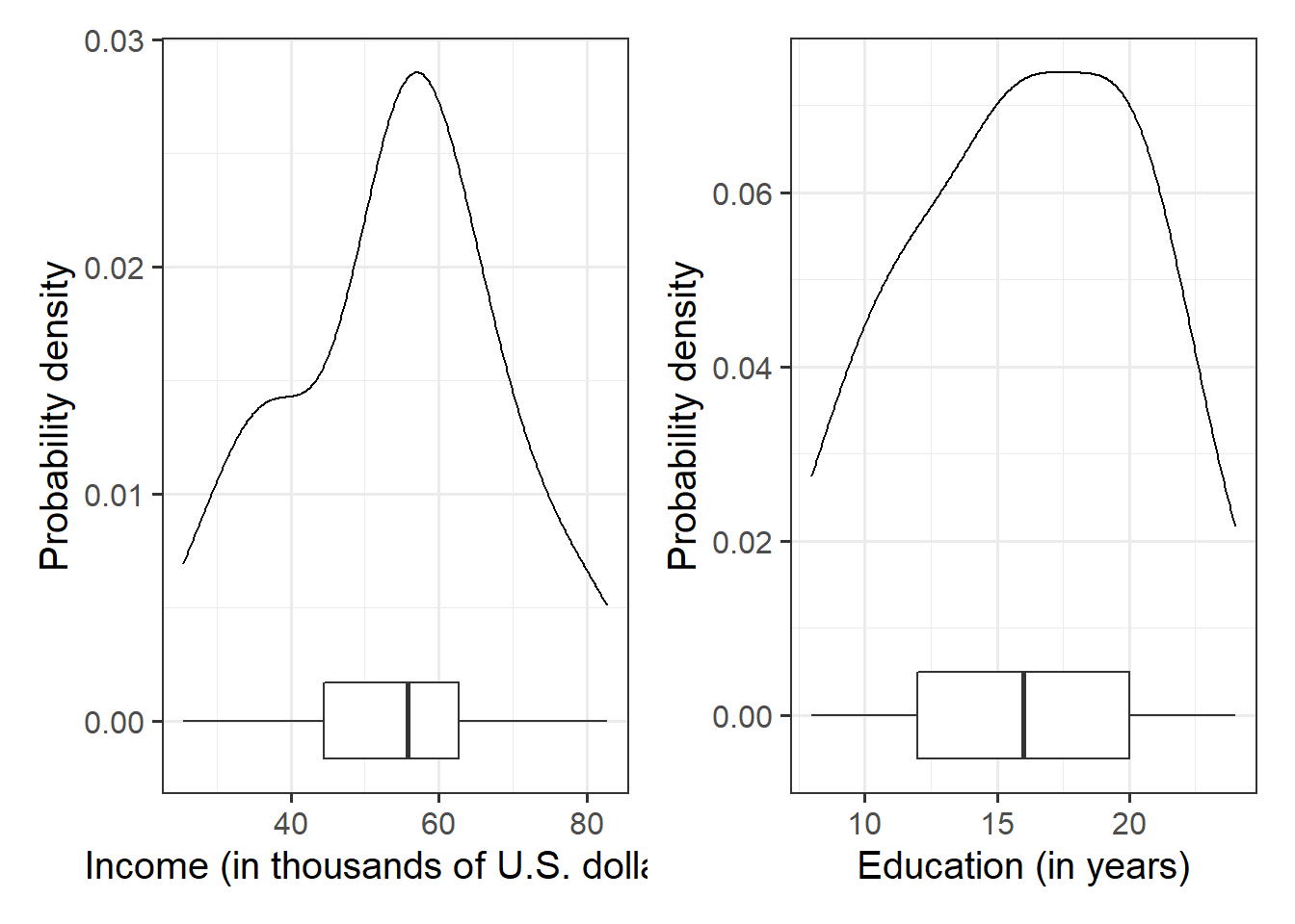
We can plot the marginal distribution of employee incomes as a density curve, and add a boxplot underneath to check for the presence of outliers. The width of the geom_boxplot() is always quite wide, so I want to make it narrower so that we can see it at the same time as the density plot. Deciding on the exact value for the width here is just trial and error:

library(patchwork)
# the patchwork library allows us to combine plots together
ggplot(data = riverview, aes(x = income)) +
  geom_density() +
  geom_boxplot(width = 1/300) +
  labs(x = "Income (in thousands of U.S. dollars)", 
       y = "Probability density") +

ggplot(data = riverview, aes(x = education)) +
  geom_density() +
  geom_boxplot(width = 1/100) +
  labs(x = "Education (in years)", 
       y = "Probability density")

Figure 1: Density plot and boxplot of employee incomes and education levels

The plots suggests that the distributions of employee incomes and education levels are both unimodal. Most of the incomes are between roughly $45,000 and $70,000, and most people have between 12 and 20 years of education. Furthermore, the boxplot does not highlight any outliers in either variable.

To further summarize a distribution, it is typical to compute and report numerical summary statistics such as the mean and standard deviation.

As we have seen, in earlier weeks, one way to compute these values is to use the summarise()/summarize() function from the tidyverse library:

riverview %>% 
  summarize(
    mean_income = mean(income), 
    sd_income = sd(income),
    mean_edu = mean(education),
    sd_edu = sd(education)
    )

# A tibble: 1 × 4
  mean_income sd_income mean_edu sd_edu
        <dbl>     <dbl>    <dbl>  <dbl>
1        53.7      14.6       16   4.36

The marginal distribution of income is unimodal with a mean of approximately $53,700. There is variation in employees’ salaries (SD = $14,553).
The marginal distribution of education is unimodal with a mean of 16 years. There is variation in employees’ level of education (SD = 4.4 years).

Question 2

After we’ve looked at the marginal distributions of the variables of interest in the analysis, we typically move on to examining relationships between the variables.

Visualise and describe the relationship between income and level of education among the employees in the sample.

Hints:
Think about:

• Direction of association
• Form of association (can it be summarised well with a straight line?)
  
• Strength of association (how closely do points fall to a recognizable pattern such as a line?)
• Unusual observations that do not fit the pattern of the rest of the observations and which are worth examining in more detail.
  

Solution

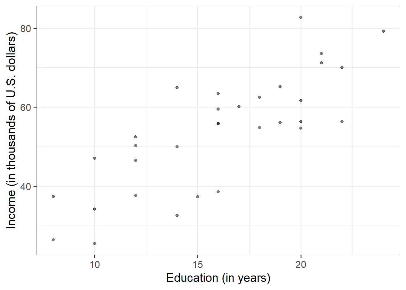
Because we are investigating how income varies when varying years of formal education, income here is the dependent variable (on the y-axis), and education is the independent variable (on the x-axis).

ggplot(data = riverview, aes(x = education, y = income)) +
  geom_point(alpha = 0.5) +
  labs(x = "Education (in years)", 
       y = "Income (in thousands of U.S. dollars)")

Figure 2: The relationship between employees education level and income.

There appears to be a strong positive linear relationship between education level and income for the employees in the sample. High incomes tend to be observed, on average, with more years of formal education. The scatterplot does not highlight any outliers.

To comment numerically on the strength of the linear association we might compute the correlation coefficient that we were introduced to in 5A: Covariance & Correlation

riverview %>%
  select(education, income) %>%
  cor()

          education    income
education 1.0000000 0.7947847
income    0.7947847 1.0000000

that is, \(r_{\text{education, income}} = 0.79\)

Question 3

Using the lm() function, fit a linear model to the sample data, in which employee income is explained by education level. Assign it to a name to store it in your environment.

Hints:
You can see how to fit linear models in R using lm() in 7A #fitting-linear-models-in-r

Solution

As the variables are in the riverview dataframe, we would write:

model1 <- lm(income ~ 1 + education, data = riverview)

Question 4

Interpret the estimated intercept and slope in the context of the question of interest.

Hints:
We saw how to extract lots of information on our model using summary() (see 7A #model-summary), but there are lots of other functions too.

If we called our linear model object “model1” in the environment, then we can use:

• type model1, i.e. simply invoke the name of the fitted model;
• type model1$coefficients;
• use the coef(model1) function;
• use the coefficients(model1) function;
• use the summary(model1)$coefficients to extract just that part of the summary.

Solution

coef(model1)

(Intercept)   education 
  11.321379    2.651297 

From this, we get that the fitted line is:

\[ \widehat{Income} = 11.32 + 2.65 \ Education \\ \]

We can interpret the estimated intercept as:

The estimated average income associated with zero years of formal education is $11,321.

For the estimated slope we get:

The estimated increase in average income associated with a one year increase in education is $2,651.

Question 5

Test the hypothesis that the population slope is zero — that is, that there is no linear association between income and education level in the population.

Hints:
You don’t need to do anything for this, you can find all the necessary information in summary() of your model.
See 7A #inference-for-regression-coefficients.

Solution

The information is already contained in the row corresponding to the variable “education” in the output of summary(), which reports the t-statistic under t value and the p-value under Pr(>|t|):

summary(model1)

Call:
lm(formula = income ~ 1 + education, data = riverview)

Residuals:
    Min      1Q  Median      3Q     Max 
-15.809  -5.783   2.088   5.127  18.379 

Coefficients:
            Estimate Std. Error t value Pr(>|t|)    
(Intercept)  11.3214     6.1232   1.849   0.0743 .  
education     2.6513     0.3696   7.173 5.56e-08 ***
---
Signif. codes:  0 '***' 0.001 '**' 0.01 '*' 0.05 '.' 0.1 ' ' 1

Residual standard error: 8.978 on 30 degrees of freedom
Multiple R-squared:  0.6317,    Adjusted R-squared:  0.6194 
F-statistic: 51.45 on 1 and 30 DF,  p-value: 5.562e-08

Recall that the p-value 5.56e-08 in the Pr(>|t|) column simply means \(5.56 \times 10^{-8}\). This is a very small value, hence we will report it as <.001 following the APA guidelines.

A significant association was found between level of education (in years) and income, with income increasing by on average $2,651 for every additional year of education (\(b = 2.65\), \(SE = 0.37\), \(t(30)=7.17\), \(p<.001\)).

Question 6

What is the proportion of the total variability in incomes explained by the linear relationship with education level?

Hints:

• The question asks to compute the value of \(R^2\), but you might be able to find it already computed somewhere (so much stuff is already in summary() of the model.
• See 7A #r2 if you’re unsure about what \(R^2\) is.

Solution

For the moment, ignore “Adjusted R-squared”. We will come back to this later on.

summary(model1)

Call:
lm(formula = income ~ 1 + education, data = riverview)

Residuals:
    Min      1Q  Median      3Q     Max 
-15.809  -5.783   2.088   5.127  18.379 

Coefficients:
            Estimate Std. Error t value Pr(>|t|)    
(Intercept)  11.3214     6.1232   1.849   0.0743 .  
education     2.6513     0.3696   7.173 5.56e-08 ***
---
Signif. codes:  0 '***' 0.001 '**' 0.01 '*' 0.05 '.' 0.1 ' ' 1

Residual standard error: 8.978 on 30 degrees of freedom
Multiple R-squared:  0.6317,    Adjusted R-squared:  0.6194 
F-statistic: 51.45 on 1 and 30 DF,  p-value: 5.562e-08

Approximately 63% of the total variability in employee incomes is explained by the linear association with education level.

Question 7

Look at the output of summary() of your model. Identify the relevant information to conduct an F-test against the null hypothesis that the model is ineffective at predicting income using education level.

Hints:
7A #the-f-statistic will help.

Solution

summary(model1)

Call:
lm(formula = income ~ 1 + education, data = riverview)

Residuals:
    Min      1Q  Median      3Q     Max 
-15.809  -5.783   2.088   5.127  18.379 

Coefficients:
            Estimate Std. Error t value Pr(>|t|)    
(Intercept)  11.3214     6.1232   1.849   0.0743 .  
education     2.6513     0.3696   7.173 5.56e-08 ***
---
Signif. codes:  0 '***' 0.001 '**' 0.01 '*' 0.05 '.' 0.1 ' ' 1

Residual standard error: 8.978 on 30 degrees of freedom
Multiple R-squared:  0.6317,    Adjusted R-squared:  0.6194 
F-statistic: 51.45 on 1 and 30 DF,  p-value: 5.562e-08

From the summary(model1), the relevant row is just below the \(R^2\), where it states:

F-statistic: 51.45 on 1 and 30 DF,  p-value: 5.562e-08

The overall test of model utility was significant \(F(1, 30) = 51.45, p < .001\), indicating evidence against the null hypothesis that the model is ineffective (that education is not a useful predictor of income).

Question 8

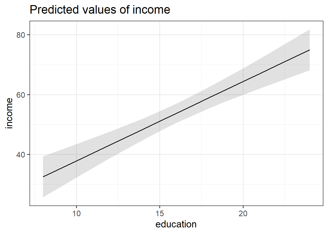
Create a visualisation of the estimated association between income and education.

Hints: Check 7A#example, which shows an example of using the sjPlot package to create a plot.

Solution

library(sjPlot)
plot_model(model1, type="eff")

$education

Optional: Question 9A

Consider the following:

1. In fitting a linear regression model, we make the assumption that the errors around the line are normally distributed around zero (this is the \(\epsilon \sim N(0, \sigma)\) bit.)
   
2. About 95% of values from a normal distribution fall within two standard deviations of the centre.

We can obtain the estimated standard deviation of the errors (\(\hat \sigma\)) from the fitted model using sigma() and giving it the name of our model.
What does this tell us?

Hints:
See 7A #the-error.

Solution

The estimated standard deviation of the errors can be obtained by:

sigma(model1)

[1] 8.978116

For any particular level of education, employee incomes should be distributed above and below the regression line with standard deviation estimated to be \(\hat \sigma = 8.98\). Since \(2 \hat \sigma = 2 (8.98) = 17.96\), we expect most (about 95%) of the employee incomes to be within about $18,000 from the regression line.

Optional: Question 9B

Compute the model-predicted income for someone with 1 year of education.

Hints:
Given that you know the intercept and slope, you can calculate this algebraically. However, try to also use the predict() function (see 7A#model-predictions).

Solution

Using predict(), we need to give it our model, plus some new data which contains a person with only 1 year of education. First we make a new dataframe with an education variable, with one entry which has the value 1, and then we give that to predict():

education_query <- data.frame(education = c(1))
predict(model1, newdata = education_query)

       1 
13.97268 

Given that our fitted model takes the form:

\[ Income = 11.32 + 2.65\cdot Education \]

We are asking what the predicted income is for someone with 1 year of education. So we can substitute in “1” for the Education variable:

\[ \begin{align} Income &= 11.32 + 2.65\cdot Education \\ Income &= 11.32 + 2.65\cdot 1 \\ Income &= 11.32 + 2.65\\ Income &= 13.97 \\ \end{align} \]

Income and Degree Status

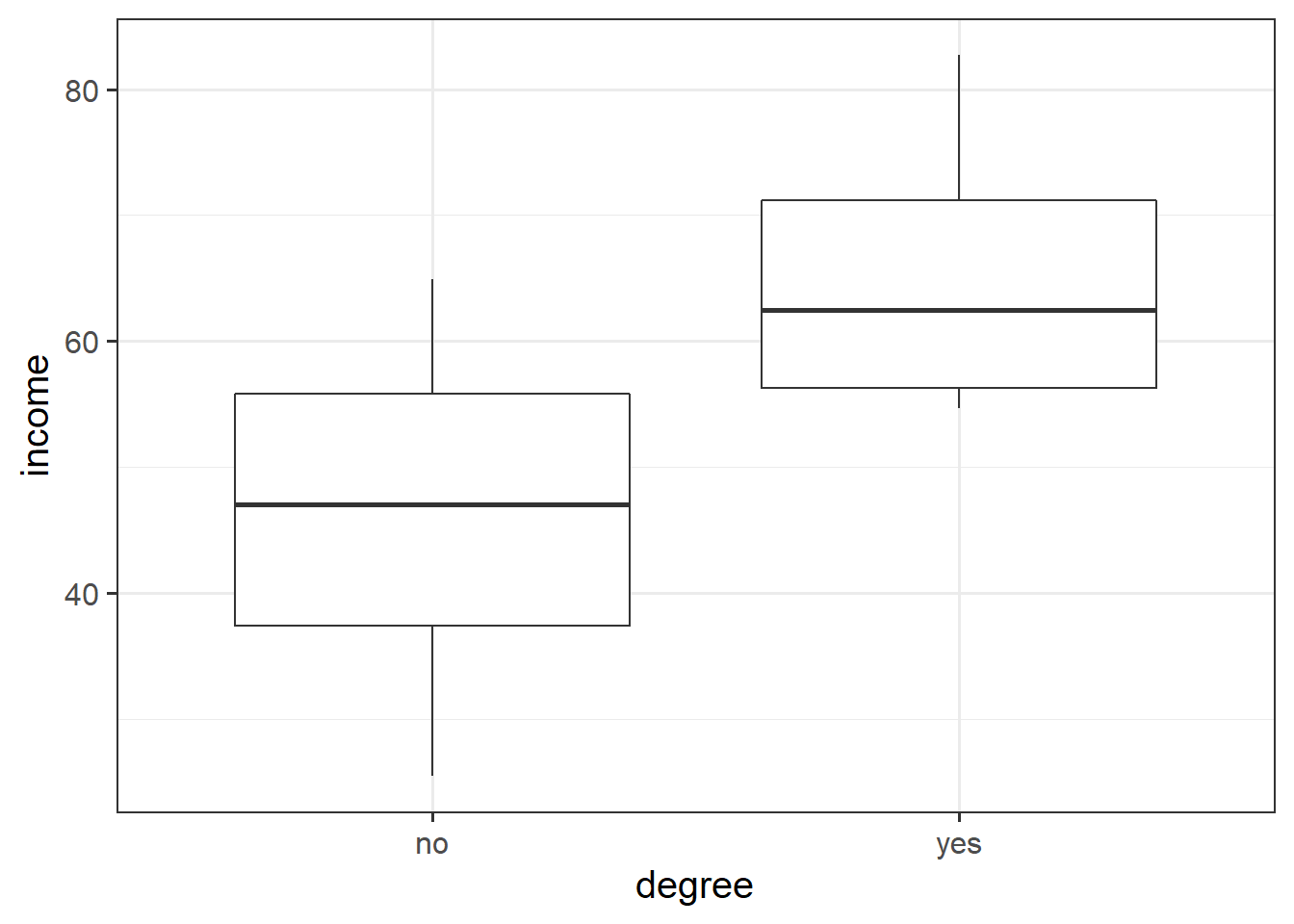
Let’s suppose instead of having measured education in years, researchers simply asked “have you had more than 18 years of education?”, assuming this to be indicative of having a degree.
The code below creates a this new variable for us:

riverview <- riverview %>%
  mutate(
    degree = ifelse(education >= 18, "yes","no")
  )

Question 10

Fit the following model, and interpret the coefficients.

\[ Income = b_0 + b_1 \ Degree + \varepsilon \]

Hints:
For help interpreting the coefficients, see 7A #binary-predictors.

Solution

model2 <- lm(income ~ degree, data = riverview)
summary(model2)

Call:
lm(formula = income ~ degree, data = riverview)

Residuals:
     Min       1Q   Median       3Q      Max 
-20.6038  -8.6706   0.3053   8.8789  18.8432 

Coefficients:
            Estimate Std. Error t value Pr(>|t|)    
(Intercept)   46.083      2.589  17.797  < 2e-16 ***
degreeyes     18.854      4.063   4.641 6.41e-05 ***
---
Signif. codes:  0 '***' 0.001 '**' 0.01 '*' 0.05 '.' 0.1 ' ' 1

Residual standard error: 11.29 on 30 degrees of freedom
Multiple R-squared:  0.4179,    Adjusted R-squared:  0.3985 
F-statistic: 21.54 on 1 and 30 DF,  p-value: 6.412e-05

• (Intercept) = the estimated income of employees without a degree (\(46,083\))
• degreeyes = the estimated change in income from employees without a degree to employees with a degree

ggplot(riverview, aes(x = degree, y = income)) +
  geom_boxplot()

Question 11

We’ve actually already seen a way to analyse questions of this sort (“is the average income different between those with and those without a degree?”)

Run the following t-test, and consider the statistic, p value etc. How does it compare to the model in the previous question?

t.test(income ~ degree, data = riverview, var.equal = TRUE)

    Two Sample t-test

data:  income by degree
t = -4.6408, df = 30, p-value = 6.412e-05
alternative hypothesis: true difference in means between group no and group yes is not equal to 0
95 percent confidence interval:
 -27.15051 -10.55673
sample estimates:
 mean in group no mean in group yes 
         46.08284          64.93646 

Solution

It is identical! the \(t\)-statistics are the same, the p-values are the same, the degrees of freedom. Everything!

The two sample t-test is actually just a special case of the linear model, where we have a numeric outcome variable and a binary predictor!

And… the one-sample t-test is the linear model without any predictors, so just with an intercept.

t.test(riverview$income, mu = 0)

    One Sample t-test

data:  riverview$income
t = 20.89, df = 31, p-value < 2.2e-16
alternative hypothesis: true mean is not equal to 0
95 percent confidence interval:
 48.49519 58.98906
sample estimates:
mean of x 
 53.74213 

interceptonly_model <- lm(income ~ 1, data = riverview)
summary(interceptonly_model)$coefficients

            Estimate Std. Error  t value     Pr(>|t|)
(Intercept) 53.74212    2.57264 20.88988 7.995568e-20

Student Sleep Quality

In the survey that many of you completed at the start of term (thank you to those that did!), we had a long set of items that were from various personality and psychometric scales.

One of these was a set of items that measure a persons’ “locus of control” (belief that you have control over your life, as opposed to it being decided by external forces such as fate/luck/destiny/god/the flying spaghetti monster). We also asked you to rate your average sleep quality from 0 to 100.

My pet theory is that people who believe they have more control over life are more inclined to have a better sleep routine, and so will rate their sleep quality as being better than those who believe that life is out of their control.

Data from the 2022 survey (now closed) can be found at https://uoepsy.github.io/data/usmr2022.csv.

usmrdata <- read_csv("https://uoepsy.github.io/data/usmr2022.csv")

The relevant variables are:

variable	description
pseudonym	User provided pseudonym to enable lookup
loc	Locus of Control Score. Minimum score = 6, maximum score = 30. Higher scores indicate more perceived self-control over life
sleeprating	Rating of average quality of sleep. Higher values indicate better sleep quality.
...	...
...	...

Question 12

Fit a linear regression model to test the association.

Hints:
Try to do the following steps:

1. Explore the data (plot and describe)
2. Fit the model
3. Take a look at the assumption plots (see 7A#assumptions).
   • The trick to looking at assumption plots is to look for “things that don’t look random”.
   • As well as looking for patterns, these plots can also higlight individual datapoints that might be skewing the results. Can you figure out if there is someone weird in our dataset? Can you re-fit the model without that person? When you do so, do your conclusions change?

Solution

usmrdata <- read_csv("https://uoepsy.github.io/data/usmr2022.csv")

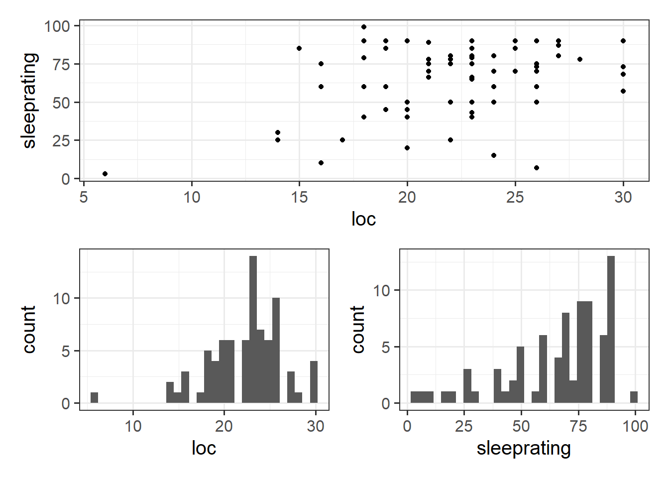
Let’s just take a look at the relevant variables and relationship:

p1 <- ggplot(usmrdata, aes(x=loc))+
  geom_histogram()
p2 <- ggplot(usmrdata, aes(x=sleeprating))+
  geom_histogram() 
p3 <- ggplot(usmrdata, aes(x=loc, y=sleeprating))+
  geom_point()
# remember, to make this plot arranging work,
# we need to load the patchwork package
p3 / (p1 + p2)

And go straight ahead and fit our model

sleepmod <- lm(sleeprating ~ loc, usmrdata)
summary(sleepmod)

Call:
lm(formula = sleeprating ~ loc, data = usmrdata)

Residuals:
    Min      1Q  Median      3Q     Max 
-66.358 -13.856   2.647  14.644  41.649 

Coefficients:
            Estimate Std. Error t value Pr(>|t|)    
(Intercept)  21.3352    13.2292   1.613 0.110892    
loc           2.0009     0.5831   3.432 0.000968 ***
---
Signif. codes:  0 '***' 0.001 '**' 0.01 '*' 0.05 '.' 0.1 ' ' 1

Residual standard error: 21.21 on 77 degrees of freedom
  (1 observation deleted due to missingness)
Multiple R-squared:  0.1326,    Adjusted R-squared:  0.1214 
F-statistic: 11.78 on 1 and 77 DF,  p-value: 0.0009681

Wooh, looks like we were right! People with greater perceived control tend to report better sleep quality.

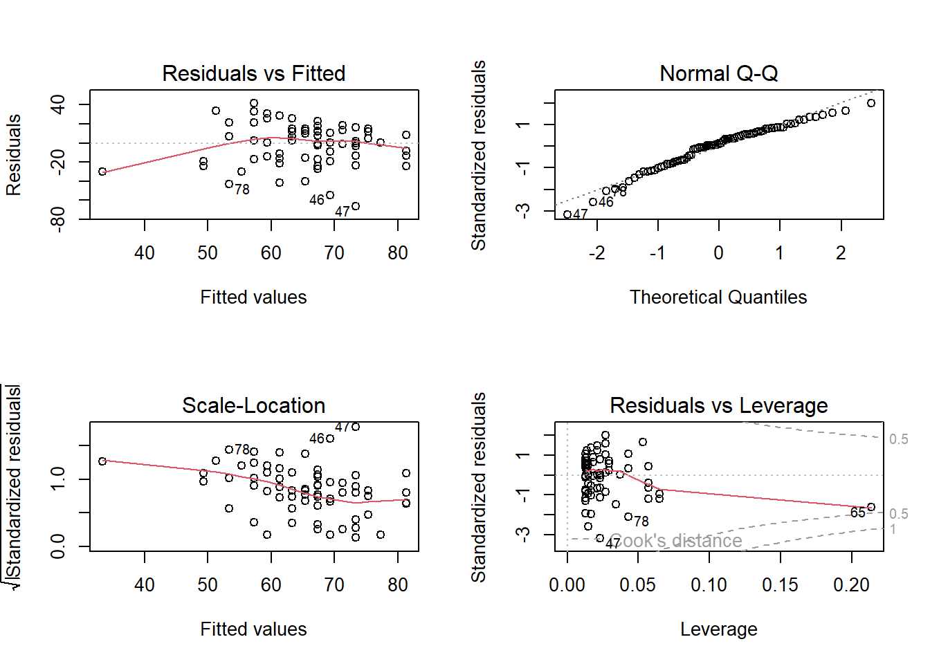
Our assumptions don’t look all that great though..

plot(sleepmod)

From the bottom right plot above, we can see that the 65th observation is looking a bit influential. There is also one datapoint that is looking weird in both of the left-hand plots - this may well be the same 65th person.
I wonder who that is..

usmrdata[65, c("pseudonym","sleeprating","loc")]

# A tibble: 1 × 3
  pseudonym          sleeprating   loc
  <chr>                    <dbl> <dbl>
1 Definitely not Ian           3     6

Ah, it’s Ian!
Ian is a guy who sleeps very badly (low sleeprating score) and feels like he has no control over his life (low loc score).
The thing is - Ian is a valuable datapoint - he’s a real person and we shouldn’t just get rid of him because he’s “a bit odd”.

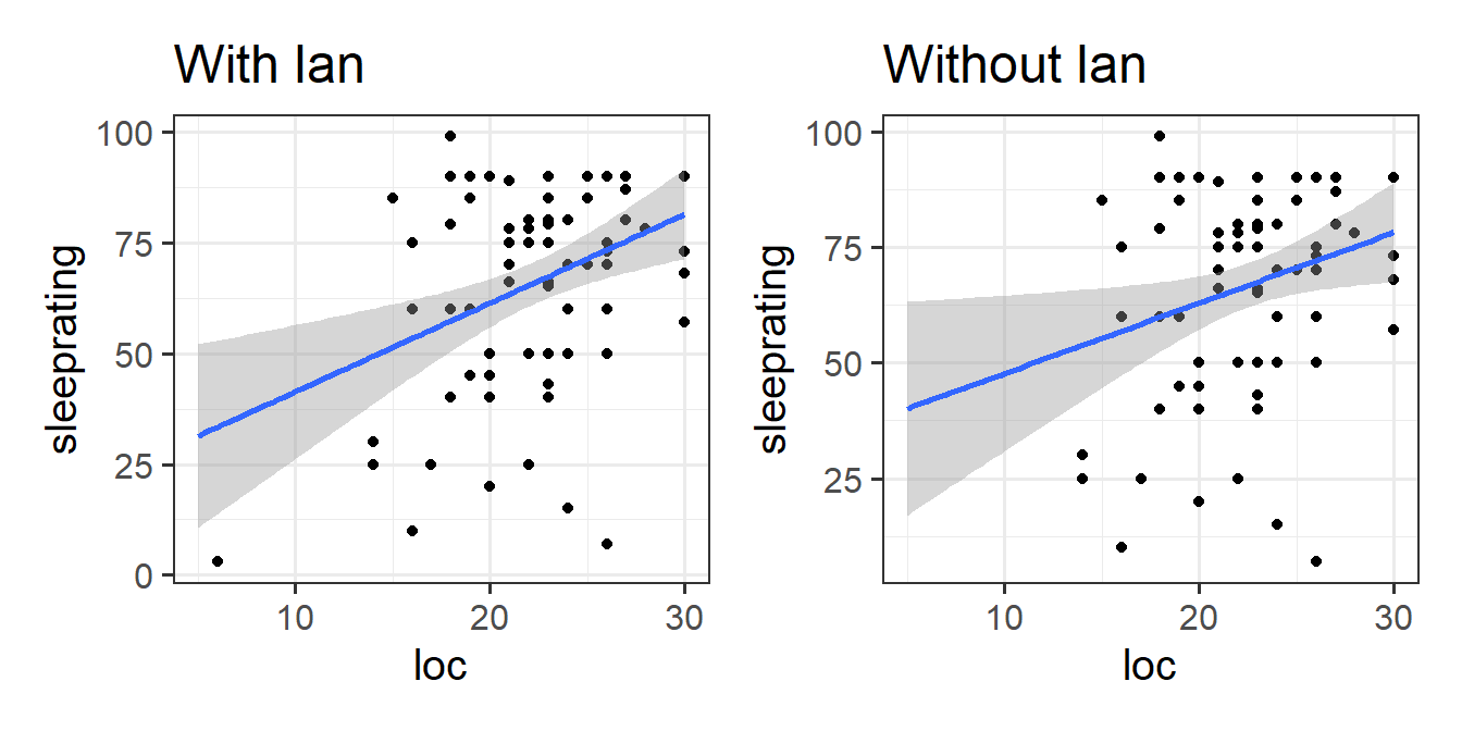
However, it would be nice to know how much Ian’s “oddness” is affecting our conclusions, so let’s re-fit the model on everybody except Ian:

sleepmod_noian <- lm(sleeprating ~ loc, usmrdata[-65, ])
summary(sleepmod_noian)

Call:
lm(formula = sleeprating ~ loc, data = usmrdata[-65, ])

Residuals:
    Min      1Q  Median      3Q     Max 
-65.093 -12.731   2.907  14.326  39.106 

Coefficients:
            Estimate Std. Error t value Pr(>|t|)  
(Intercept)  32.4454    14.7558   2.199   0.0309 *
loc           1.5249     0.6465   2.359   0.0209 *
---
Signif. codes:  0 '***' 0.001 '**' 0.01 '*' 0.05 '.' 0.1 ' ' 1

Residual standard error: 20.98 on 76 degrees of freedom
  (1 observation deleted due to missingness)
Multiple R-squared:  0.06821,   Adjusted R-squared:  0.05595 
F-statistic: 5.563 on 1 and 76 DF,  p-value: 0.02091

Our conclusions haven’t changed - we still have a significant association.

What we have just done is called a “sensitivity analysis” - we’ve asked if our analyses are sensitive to including/excluding Ian.

Code

ggplot(usmrdata, aes(x=loc,y=sleeprating))+
  geom_point()+
  geom_smooth(method=lm, fullrange=TRUE)+
  xlim(5,30)+
  labs(title="With Ian") +

ggplot(usmrdata[-65, ], aes(x=loc,y=sleeprating))+
  geom_point()+
  geom_smooth(method=lm, fullrange=TRUE)+
  xlim(5,30)+
  labs(title="Without Ian")

We now have a decision to make. Do we continue with Ian removed, or do we keep him in? There’s not really a right answer here, but it’s worth noting a practical issue - our assumption plots look considerably better¹ for our model without Ian.

Personally, I would probably remove Ian, and when writing up the analysis, mention clearly why we exclude him, and how that decision has/hasn’t influenced our conclusions.

Footnotes

1. Still not perfect, but don’t worry about that right now