Week 9 Exercises: Interactions and Categorical Predictors

Aging Cognition

Data: cogapoe4.csv

Ninety adult participants were recruited for a study investigating how cognitive functioning varies by age, and whether this is different depending on whether people carry an APOE-4 gene.

Research Question: Does the relationship between age and cognitive functioning differ between those with and without the APOE-4 genotype?

The data are available at https://uoepsy.github.io/data/cogapoe4.csv.

variables	description
pid	Participant ID
age	Age (in Years)
educ	Years of Education
birthweight_kg	Birthweight (in Kg)
apoe4	APOE-4 Gene expansion ('none', 'apoe4a', 'apoe4b', apoe4c')
acer	Score on Addenbrooke's Cognitive Examination

Question 1

Does the relationship between age and cognitive functioning differ between those with and without the APOE-4 genotype?

Read in the data and explore the variables which you think you will use to answer the research question above (create some plots, some descriptive stats etc.)

handy functions:

• The pairs.panels() function from the psych package is quite a nice way to plot a scatterplot matrix of a dataset.
  
• The describe() function is also quite nice (from the psych package too).

cogapoe <- read_csv("https://uoepsy.github.io/data/cogapoe4.csv")
summary(cogapoe)

     pid                 age              educ       birthweight_kg  
 Length:90          Min.   : 45.00   Min.   :15.00   Min.   : 0.500  
 Class :character   1st Qu.: 57.25   1st Qu.:17.00   1st Qu.: 5.225  
 Mode  :character   Median : 67.00   Median :19.00   Median : 6.550  
                    Mean   : 70.53   Mean   :19.31   Mean   : 6.546  
                    3rd Qu.: 86.75   3rd Qu.:22.00   3rd Qu.: 8.150  
                    Max.   :100.00   Max.   :24.00   Max.   :11.500  
    apoe4                acer       
 Length:90          Min.   : 70.42  
 Class :character   1st Qu.: 78.52  
 Mode  :character   Median : 85.02  
                    Mean   : 86.53  
                    3rd Qu.: 95.36  
                    Max.   :100.00  

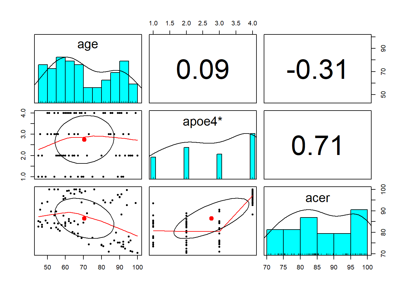
Judging by the research question, we’re going to be interested in participants’ ages, whether they carry the APOE4 gene, and their cognitive functioning.

library(psych)

cogapoe %>% 
  select(age, apoe4, acer) %>%
  pairs.panels()

cogapoe %>% 
  select(age, apoe4, acer) %>%
  describe()

       vars  n  mean    sd median trimmed   mad   min max range  skew kurtosis
age       1 90 70.53 16.28  67.00   70.28 19.27 45.00 100 55.00  0.21    -1.30
apoe4*    2 90  2.76  1.13   3.00    2.82  1.48  1.00   4  3.00 -0.25    -1.40
acer      3 90 86.53  9.39  85.02   86.63 13.11 70.42 100 29.58 -0.01    -1.34
         se
age    1.72
apoe4* 0.12
acer   0.99

Question 2

Check the apoe4 variable. It currently has four levels (“none”/“apoe4a”/“apoe4b”/“apoe4c”), but the research question is actually interested in two (“none” vs “apoe4”).

Make a new variable that indicates whether or not someone has the APOE4 genotype.

Hints:

• One way to do this would be to use ifelse() to define a variable which takes one value (e.g., “NO”) if the observation meets from some condition, or another value (e.g., “YES”) if it does not. You can use it to add a new variable either inside mutate(), or using data$new_variable_name <- ifelse(test, x, y) syntax.

Create a new variable for APOE4 Yes or No

cogapoe <- 
  cogapoe %>% 
  mutate(
    isAPOE4 = ifelse(apoe4 == "none", "No", "Yes")
  )

Question 3

Does the relationship between age and cognitive functioning differ between those with and without the APOE-4 genotype?

To answer this question, do you need an interaction? If so, between what kind of variables (continuous x continuous, continuous x categorical, or categorical x categorical)?

Hint:

• See 9A#it-depends

Does the relationship between [continuous predictor] and [outcome] differ between [categorical predictor]?

It’s continuous x categorical!

Question 4

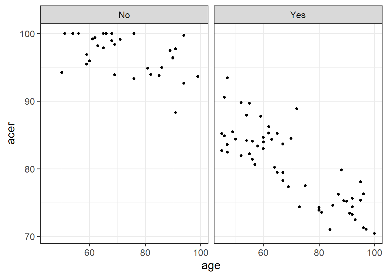
Especially for this type of interactions, we can start to get a sense of things by plotting the data and having a separate facet for each group.

Produce a visualisation of the relationship between age and cognitive functioning, with separate facets for people with and without the APOE4 gene.

Hint:

• remember facet_wrap()?

ggplot(data = cogapoe, aes(x = age, y = acer)) + 
  geom_point() + 
  facet_wrap(~isAPOE4)

Question 5

Does the relationship between age and cognitive functioning differ between those with and without the APOE-4 genotype?

Fit a model to answer this research question.

Hint:

• for how to fit interactions, see 9A#fitting-interactions-in-r

apoe4mod <- lm(acer ~ 1 + age * isAPOE4, data = cogapoe)

Question 6

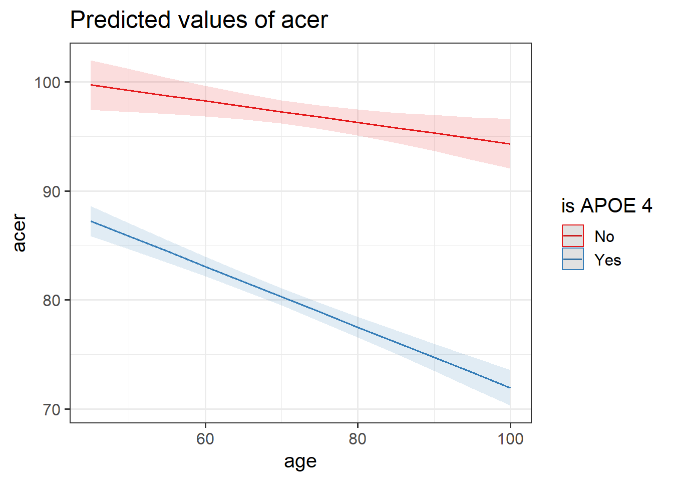
Looking at the coefficient estimates from your model, write a description of what each one corresponds to on the plot shown in Figure 1 (it may help to sketch out the plot yourself and annotate it).

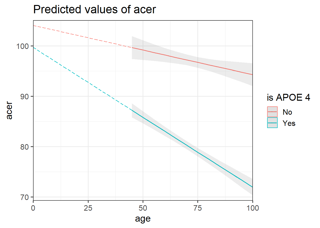
Figure 1: Multiple regression model: ACER ~ Age * isAPOE4
The dotted lines show the extension back to where the x-axis is zero

Some options for you to choose from:

• The point at which the blue line cuts the y-axis (where age = 0)
• The point at which the red line cuts the y-axis (where age = 0)
• The average vertical distance between the red and blue lines.
• The vertical distance from the blue to the red line at the y-axis (where age = 0)
• The vertical distance from the red to the blue line at the y-axis (where age = 0)
• The vertical distance from the blue to the red line at the center of the plot
• The vertical distance from the red to the blue line at the center of the plot
• The slope (vertical increase on the y-axis associated with a 1 unit increase on the x-axis) of the blue line
• The slope of the red line
• The adjustment to the slope when you move from the blue to the red line
• The adjustment to the slope when you move from the red to the blue line

As always, we can obtain our coefficient estimates using various functions such as summary(apoe4mod),coef(apoe4mod), coefficients(apoe4mod) etc.

coefficients(apoe4mod)

   (Intercept)            age     isAPOE4Yes age:isAPOE4Yes 
  104.09765349    -0.09796756    -4.37223106    -0.17966769 

• (Intercept) = 104.1: The point at which the red line cuts the y-axis (where age = 0).
  
• age = -0.1: The slope (vertical change on the y-axis associated with a 1 unit change on the x-axis) of the red line.
• isAPOE4Yes = -4.37: The vertical distance from the red to the blue line at the y-axis (where age = 0).
  
• age:isAPOE4Yes = -0.18: How the slope of the line changes when you move from the red to the blue line.

Question 7

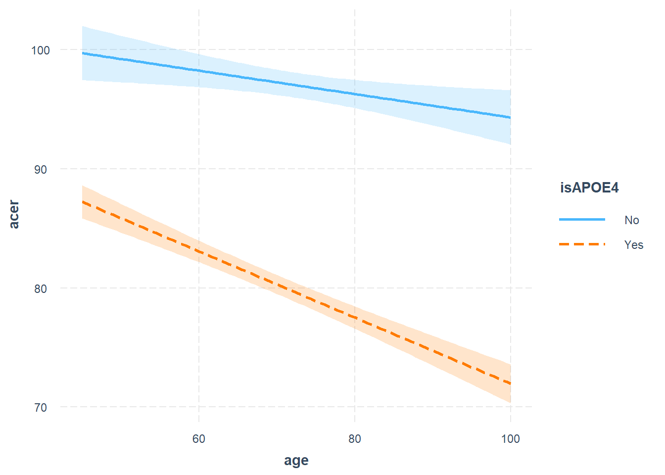
Produce a visualisation of the estimated interaction.

Hints:

• e.g. plot your model!
• see 9A#visualisation

If we use sjPlot:

library(sjPlot)
plot_model(apoe4mod, type="int")

Or interactions:

library(interactions)
interact_plot(apoe4mod, pred = "age", modx="isAPOE4", interval = TRUE)

Question 8

Write a short paragraph explaining the pattern of results, including coefficient estimates as appropriate.

summary(apoe4mod)

Call:
lm(formula = acer ~ 1 + age * isAPOE4, data = cogapoe)

Residuals:
    Min      1Q  Median      3Q     Max 
-6.8923 -2.1408 -0.0917  2.0802  9.1208 

Coefficients:
                Estimate Std. Error t value Pr(>|t|)    
(Intercept)    104.09765    2.72786  38.161  < 2e-16 ***
age             -0.09797    0.03689  -2.655  0.00944 ** 
isAPOE4Yes      -4.37223    3.20121  -1.366  0.17556    
age:isAPOE4Yes  -0.17967    0.04372  -4.110 9.01e-05 ***
---
Signif. codes:  0 '***' 0.001 '**' 0.01 '*' 0.05 '.' 0.1 ' ' 1

Residual standard error: 3.025 on 86 degrees of freedom
Multiple R-squared:  0.8996,    Adjusted R-squared:  0.8961 
F-statistic:   257 on 3 and 86 DF,  p-value: < 2.2e-16

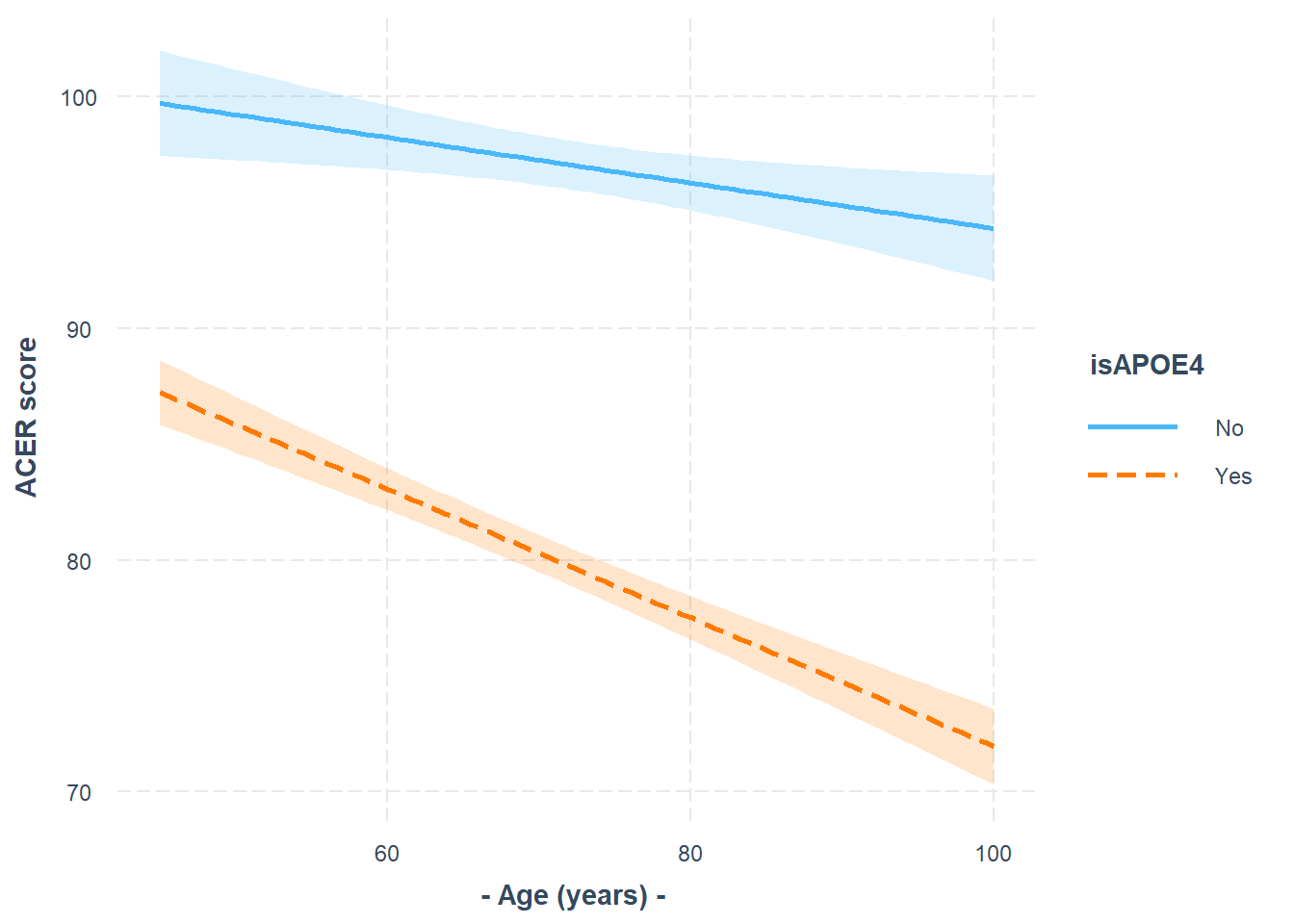
For those without the APOE4 gene, the estimated average score on the ACER was found to decrease by 0.1 points with every year of age (\(\beta = -0.1\), \(t(86) = -2.66\), \(p <0.05\)). A significant interaction between age and APOE4 status indicates that those with the APOE4 gene have an decline by 0.18 more for every year of age than those without the gene (\(\beta = -0.18\), \(t(86) = -4.11\), \(p <0.05\)). This is visualised in Figure 2.

Figure 2: Decreases in cognition depend upon APOE4 genotype

Question 9

It’s important to emphasise that models are structures that we design, then estimate from our data, and assess how well they fit.

Here are three models:

cogapoe$isAPOE4 = ifelse(cogapoe$apoe4 == "none", "No", "Yes")
apoe4mod1 <- lm(acer ~ 1 + age, data = cogapoe)
apoe4mod2 <- lm(acer ~ 1 + age + isAPOE4, data = cogapoe)
apoe4mod3 <- lm(acer ~ 1 + age + isAPOE4 + age:isAPOE4, data = cogapoe)

And below are those three models plotted, with the data added.
Which model corresponds to which plot?

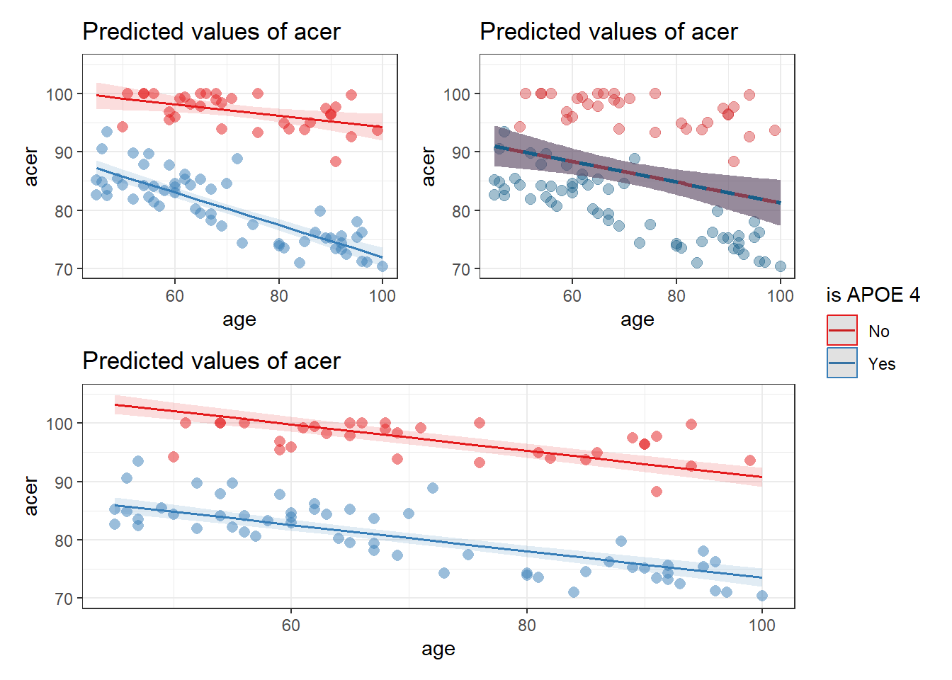
The top left shows non-parallel lines. It’s an interaction! This is the model acer ~ 1 + age + isAPOE4 + age:isAPOE4.

The top right shows no estimated differences in ACER scores between APOE4 positive and negative. This is probably the model acer ~ 1 + age, where APOE4 isn’t in the model at all.

The bottom shows two parallel lines. They differ in height, so there is an estimated association between APOE4 and ACER scores. The lines being parallel means this will be the one without an interaction acer ~ 1 + age + isAPOE4.

If you fit a model with an interaction in it, you don’t always get non-parallel lines. If the interaction coefficient is 0 (and so non-significant), then the model would look like two parallel lines.

Personality and Social Rank

Data: scs_study.csv

Data from 656 participants containing information on scores on each trait of a Big 5 personality measure, their perception of their own social rank, and their scores on a measure of depression. Previous research has identified an association between an individual’s perception of their social rank and symptoms of depression, anxiety and stress. We are interested in the individual differences in this relationship.

Research Question: After accounting for other personality traits, does the effect of social comparison on symptoms of depression, anxiety and stress vary depending on level of neuroticism?

The data is available at https://uoepsy.github.io/data/scs_study.csv.

The data in scs_study.csv contain seven attributes collected from a random sample of \(n=656\) participants:

• zo: Openness (Z-scored), measured on the Big-5 Aspects Scale (BFAS)
• zc: Conscientiousness (Z-scored), measured on the Big-5 Aspects Scale (BFAS)
• ze: Extraversion (Z-scored), measured on the Big-5 Aspects Scale (BFAS)
• za: Agreeableness (Z-scored), measured on the Big-5 Aspects Scale (BFAS)
• zn: Neuroticism (Z-scored), measured on the Big-5 Aspects Scale (BFAS)
• scs: Social Comparison Scale - An 11-item scale that measures an individual’s perception of their social rank, attractiveness and belonging relative to others. The scale is scored as a sum of the 11 items (each measured on a 5-point scale), with higher scores indicating more favourable perceptions of social rank. Scores range from 11 to 55.
  
• dass: Depression Anxiety and Stress Scale - The DASS-21 includes 21 items, each measured on a 4-point scale. The score is derived from the sum of all 21 items, with higher scores indicating higher a severity of symptoms. Scores range from 21 to 84.

What does ‘Z-scored’ mean?

“Z-scoring” is a method of standardising a variable so that it has a mean of zero and a standard deviation of one. We actually saw this back in 2B#the-standard-normal-distribution.

To transform a given value \(x_i\) into a z-score \(z_i\), we simply calculate the distance from \(x_i\) to the mean, \(\bar{x}\), and divide this by the standard deviation, \(s\):
\[ z_i = \frac{x_i - \bar{x}}{s} \]

A Z-score of a value is the number of standard deviations below/above the mean that the value falls.

Question 10

Read in the Social Comparison Study data and explore the relevant distributions and relationships between the variables of interest to the research question below.

After accounting for other personality traits, does the effect of social comparison on symptoms of depression, anxiety and stress vary depending on level of neuroticism?

scs_study <- read_csv("https://uoepsy.github.io/data/scs_study.csv")
summary(scs_study)

       zo                 zc                 ze                 za          
 Min.   :-2.81928   Min.   :-3.21819   Min.   :-3.00576   Min.   :-2.94429  
 1st Qu.:-0.63089   1st Qu.:-0.66866   1st Qu.:-0.68895   1st Qu.:-0.69394  
 Median : 0.08053   Median : 0.00257   Median :-0.04014   Median :-0.01854  
 Mean   : 0.09202   Mean   : 0.01951   Mean   : 0.00000   Mean   : 0.00000  
 3rd Qu.: 0.80823   3rd Qu.: 0.71215   3rd Qu.: 0.67085   3rd Qu.: 0.72762  
 Max.   : 3.55034   Max.   : 3.08015   Max.   : 2.80010   Max.   : 2.97010  
       zn               scs             dass      
 Min.   :-1.4486   Min.   :27.00   Min.   :23.00  
 1st Qu.:-0.7994   1st Qu.:33.00   1st Qu.:41.00  
 Median :-0.2059   Median :35.00   Median :44.00  
 Mean   : 0.0000   Mean   :35.77   Mean   :44.72  
 3rd Qu.: 0.5903   3rd Qu.:38.00   3rd Qu.:49.00  
 Max.   : 3.3491   Max.   :54.00   Max.   :68.00  

p1 <- ggplot(data = scs_study, aes(x=dass)) + 
  geom_density() + 
  geom_boxplot(width = 1/50) +
  labs(title="Marginal distribution of DASS-21 Scores", 
       x = "Depression Anxiety and Stress Scale", y = "Probability density")

p2 <- ggplot(data = scs_study, aes(x=scs)) + 
  geom_density() + 
  geom_boxplot(width = 1/50) +
  labs(title="Marginal distribution of Social Comparison Scale (SCS) scores", 
       x = "Social Comparison Scale Score", y = "Probability density")

p3 <- ggplot(data = scs_study, aes(x=zn)) + 
  geom_density() + 
  geom_boxplot(width = 1/50) +
  labs(title="Marginal distribution of Neuroticism (Z-Scored)", 
       x = "Neuroticism (Z-Scored)", y = "Probability density")
library(patchwork)
p1 / (p2 + p3)

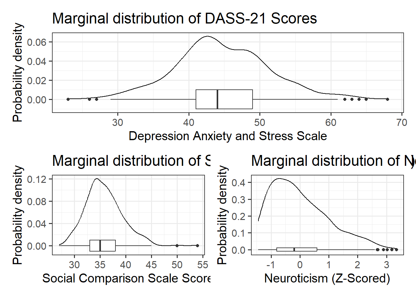
The marginal distribution of scores on the Depression, Anxiety and Stress Scale (DASS-21) is unimodal with a mean of approximately 45 and a standard deviation of 7.

The marginal distribution of scores on the Social Comparison Scale (SCS) is unimodal with a mean of approximately 36 and a standard deviation of 4. There look to be a number of outliers at the upper end of the scale.

The marginal distribution of Neuroticism (Z-scored) is positively skewed, with the 25% of scores falling below -0.8, 75% of scores falling below 0.59.

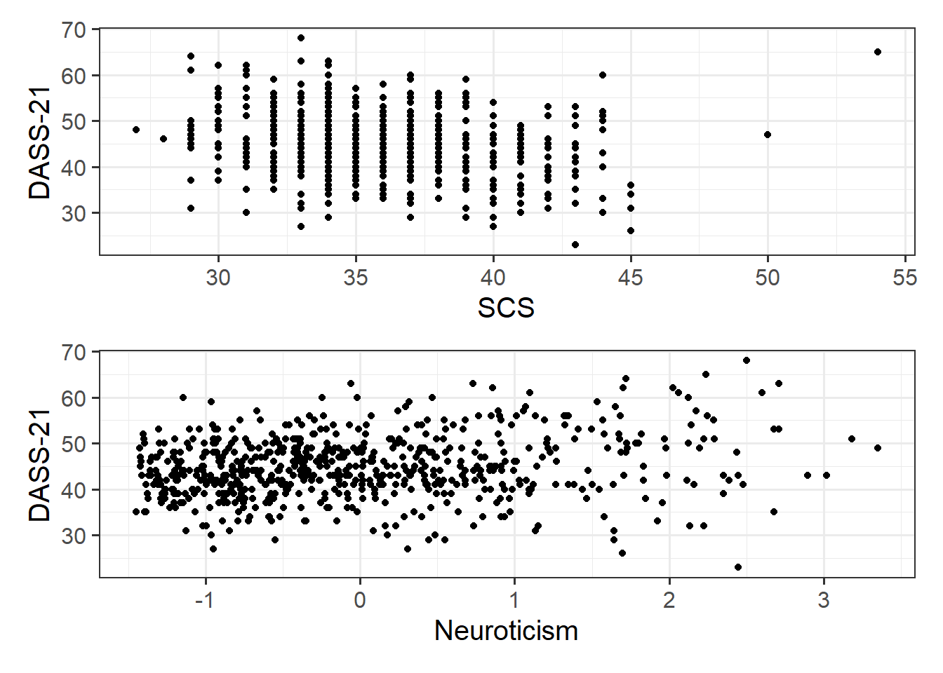
p1 <- ggplot(data = scs_study, aes(x=scs, y=dass)) + 
  geom_point()+
  labs(x = "SCS", y = "DASS-21")

p2 <- ggplot(data = scs_study, aes(x=zn, y=dass)) + 
  geom_point()+
  labs(x = "Neuroticism", y = "DASS-21")

p1 / p2

library(knitr) # for making tables look nice
# the kable() function from the knitr package can make table outputs print nicely into html.
scs_study %>%
  select(dass, scs, zn) %>%
  cor %>% 
  kable

	dass	scs	zn
dass	1.0000000	-0.2280126	0.2001885
scs	-0.2280126	1.0000000	0.1146687
zn	0.2001885	0.1146687	1.0000000

There is a weak, negative, linear relationship between scores on the Social Comparison Scale and scores on the Depression Anxiety and Stress Scale for the participants in the sample. Severity of symptoms measured on the DASS-21 tend to decrease, on average, the more favourably participants view their social rank.
There is a weak, positive, linear relationship between the levels of Neuroticism and scores on the DASS-21. Participants who are more neurotic tend to, on average, display a higher severity of symptoms of depression, anxiety and stress.

Question 11

Fit your model using lm(). Examine the coefficients, plot the relevant estimated associations to visually address the research question.

Hints:

• there are sort of two bits to this:
  • “after accounting for” (i.e., the stuff we learned in 8A#multiple-regression)
  • “the effect of this depends on that” (the interaction stuff from 9a#interactions).

dass_mdl <- lm(dass ~ 1 + zo + zc + ze + za + scs*zn, data = scs_study)
summary(dass_mdl)

Call:
lm(formula = dass ~ 1 + zo + zc + ze + za + scs * zn, data = scs_study)

Residuals:
    Min      1Q  Median      3Q     Max 
-17.346  -3.817  -0.195   3.865  45.214 

Coefficients:
            Estimate Std. Error t value Pr(>|t|)    
(Intercept) 60.83961    2.44077  24.926  < 2e-16 ***
zo          -0.18341    0.23322  -0.786   0.4319    
zc          -0.05606    0.23795  -0.236   0.8138    
ze           0.72317    0.36203   1.998   0.0462 *  
za           0.19870    0.36289   0.548   0.5842    
scs         -0.44425    0.06798  -6.535 1.29e-10 ***
zn          20.13823    2.34987   8.570  < 2e-16 ***
scs:zn      -0.51957    0.06524  -7.964 7.48e-15 ***
---
Signif. codes:  0 '***' 0.001 '**' 0.01 '*' 0.05 '.' 0.1 ' ' 1

Residual standard error: 6.075 on 648 degrees of freedom
Multiple R-squared:  0.2002,    Adjusted R-squared:  0.1916 
F-statistic: 23.17 on 7 and 648 DF,  p-value: < 2.2e-16

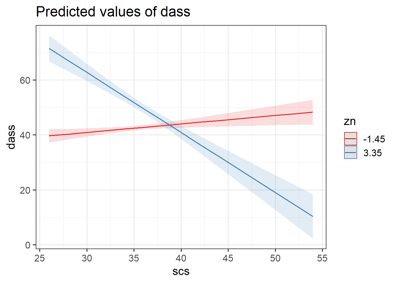
Recall that the coefficient zn from our model now reflects the estimated change in the outcome associated with an increase of 1 in neuroticism, when the other variable (SCS) is zero (and holding constant other personality traits).

plot_model(dass_mdl, type = "int")

Question 12

Think - what does “0” represent in each variable? And what does an increase of 1 represent? Are these meaningful?

The zn variable is standardised, meaning that “0” is the mean, and moving from “0” to “1” is moving 1 standard deviation.

I would argue that because “0” on scs variable is not a possible score that anyone can get, we may want to re-center this variable.

Recenter the scs variable on either:

• the minimum possible SCS score
• the mean SCS score

Hint:

• You can choose either min or mean. It won’t change your model, it will just change what you get out of it.
  
• You can see an example of mean-centering in 9A#getting-more-from-your-model.

scs_study <-
  scs_study %>%
  mutate(
    scs_Cmean = scs - mean(scs),
    scs_Cmin = scs - min(scs)
  )

Question 13

Re-fit your model using your re-centered SCS scores instead of the original variable.

Fill in the blanks in the statements below.

• For those at the mean on all personality traits and scoring ??? on the SCS, the estimated DASS-21 Score is ???
  
• For those who score ??? on the SCS, an increase of ??? in neuroticism is associated with a change of ??? in DASS-21 Scores, holding other personality traits constant.
• For those of average neuroticism, an increase of ??? on the SCS is associated with a change of ??? in DASS-21 Scores, holding other personality traits constant.
  
• For every increase of ??? in neuroticism, the change in DASS-21 associated with an increase of ??? on the SCS is asjusted by ???
• For every increase of ??? in SCS, the change in DASS-21 associated with an increase of ??? in neuroticism is asjusted by ???

Mean Centered

dass_mdl2 <- lm(dass ~ 1 + scs_Cmean * zn, data = scs_study)
# pull out the coefficients from the summary():
summary(dass_mdl2)$coefficients

               Estimate Std. Error    t value     Pr(>|t|)
(Intercept)  44.9324476 0.24052861 186.807079 0.000000e+00
scs_Cmean    -0.4439065 0.06834135  -6.495431 1.643265e-10
zn            1.5797687 0.24086372   6.558766 1.105118e-10
scs_Cmean:zn -0.5186142 0.06552100  -7.915236 1.063297e-14

• For those at the mean on all personality traits and scoring average on the SCS, the estimated DASS-21 Score is 44.93
  
• For those who score average (mean) on the SCS, an increase of 1 standard deviation in neuroticism is associated with a change of 1.58 in DASS-21 Scores, holding other personality traits constant.
• For those of average neuroticism, an increase of 1 point on the SCS is associated with a change of -0.44 in DASS-21 Scores, holding other personality traits constant.
  
• For every increase of 1 standard deviation in neuroticism, the change in DASS-21 associated with an increase of 1 point on the SCS is asjusted by -0.52
• For every increase of 1 point in SCS, the change in DASS-21 associated with an increase of 1 standard deviation in neuroticism is asjusted by -0.52

Minimum-centered

dass_mdl2a <- lm(dass ~ 1 + scs_Cmin * zn, data = scs_study)
# pull out the coefficients from the summary():
summary(dass_mdl2a)$coefficients

              Estimate Std. Error   t value     Pr(>|t|)
(Intercept) 48.8233968 0.64359279 75.860695 0.000000e+00
scs_Cmin    -0.4439065 0.06834135 -6.495431 1.643265e-10
zn           6.1255486 0.62628048  9.780839 3.572450e-21
scs_Cmin:zn -0.5186142 0.06552100 -7.915236 1.063297e-14

• For those at the mean on all personality traits and scoring minimum on the SCS, the estimated DASS-21 Score is 48.82
  
• For those who score the minimum on the SCS, an increase of 1 standard deviation in neuroticism is associated with a change of 6.13 in DASS-21 Scores, holding other personality traits constant.
• For those of average neuroticism, an increase of 1 point on the SCS is associated with a change of -0.44 in DASS-21 Scores, holding other personality traits constant.
  
• For every increase of 1 standard deviation in neuroticism, the change in DASS-21 associated with an increase of 1 point on the SCS is asjusted by -0.52
• For every increase of 1 point in SCS, the change in DASS-21 associated with an increase of 1 standard deviation in neuroticism is asjusted by -0.52

Seasonal Extraversion

USMR 2022 Data

The data from the USMR 2022 survey (now closed) can be found at https://uoepsy.github.io/data/usmr2022.csv.

note, this is the survey data just from USMR this year, not other students on other courses or in previous years

Question 14

We want to make a variable that indicates what season each person was born in.

We have seen the ifelse() command a few of times now, but something we are yet to see is that we can have nested statements. So we could turn everybody’s birth-months into a season by doing something like the below, where we ask “if it’s january then it’s winter, else if it’s february then it’s winter, else if it’s march…” and so on.

usmrdata <- read_csv("https://uoepsy.github.io/data/usmr2022.csv")
usmrdata %>% mutate(
  season = ifelse(birthmonth == "jan", "winter",
                  ifelse(birthmonth == "feb", "winter",
                         ifelse(birthmonth == "mar", "spring"
                                ifelse( ..... 
)

We can make this a little more efficient by use of the %in% operator, which allows us to ask “if it’s one of [december, january, february] then it’s winter, else…”.

usmrdata %>% mutate(
  season = ifelse(birthmonth %in% c("dec","jan", "feb"), "winter",
                  ifelse(birthmonth %in% c("mar","apr","may"), "spring",
                         ...
                         ...
)

Complete the code above in order to make a column that assigns the correct birth-season based on their month of birth.

Hints:

• you don’t have to write out the last “if”, because you can capture those in the final “else” bit.
  
• if you want a more tidyverse way to do this then look up the help docs for the case_when() function.

usmrdata <- read_csv("https://uoepsy.github.io/data/usmr2022.csv")

usmrdata <- 
  usmrdata %>% 
  mutate(
    season = ifelse(birthmonth %in% c("dec","jan", "feb"), "winter",
                  ifelse(birthmonth %in% c("mar","apr","may"), "spring",
                         ifelse(birthmonth %in% c("jun","jul","aug"), "summer",
                                "autumn")))
  )

The tidyverse way:

usmrdata <- 
  usmrdata %>% 
  mutate(
    season = case_when(
      birthmonth %in% c("dec","jan", "feb") ~ "winter",
      birthmonth %in% c("mar","apr","may") ~ "spring",
      birthmonth %in% c("jun","jul","aug") ~ "summer",
      TRUE ~ "autumn"
    )
  )

Question 15

Make the season variable that you just created a factor.

We would like you to do the following, in order:

1. fit a model lm(extraversion ~ season), and assign it the name seasonmod1.
   
2. relevel the season variable to have “spring” as the reference level.
3. fit the same model, this time assigning it the name seasonmod2
4. set the contrasts for the season variable to be “sum contrasts”
5. fit the same model, this time assigning it the name seasonmod3

Hints:

• for relevelling factors, we’ve seen this in 9A#getting-more-from-your-model.
• for “sum contrasts” and how to set them, see 9B#sum-contrasts.

Make it a factor:

usmrdata$season <- factor(usmrdata$season)

fit model 1

seasonmod1 <- lm(extraversion ~ season, data = usmrdata)

relevel to have spring as the reference:

usmrdata$season <- fct_relevel(usmrdata$season, "spring")

fit model again (model 2)

seasonmod2 <- lm(extraversion ~ season, data = usmrdata)

here are the current contrasts:

contrasts(usmrdata$season)

       autumn summer winter
spring      0      0      0
autumn      1      0      0
summer      0      1      0
winter      0      0      1

set them to sum contrasts:

contrasts(usmrdata$season) <- "contr.sum"

and take a look

contrasts(usmrdata$season)

       [,1] [,2] [,3]
spring    1    0    0
autumn    0    1    0
summer    0    0    1
winter   -1   -1   -1

fit the model again (model 3)

seasonmod3 <- lm(extraversion ~ season, data = usmrdata)

Question 16

Calculate the mean extraversion of people born in each season. From these, also calculate the mean of those four means.

Hints:

• you can use the data %>% group_by %>% summarise logic here.
  
• to calculate a mean of means, how about data %>% group_by %>% summarise %>% summarise!

usmrdata %>%
  group_by(season) %>%
  summarise(meanEx = mean(extraversion))

# A tibble: 4 × 2
  season meanEx
  <fct>   <dbl>
1 spring   30.3
2 autumn   26.1
3 summer   33.2
4 winter   29.7

usmrdata %>%
  group_by(season) %>%
  summarise(meanEx = mean(extraversion)) %>%
  summarise(grandmeanEx = mean(meanEx))

# A tibble: 1 × 1
  grandmeanEx
        <dbl>
1        29.8

Question 17

Because there aren’t any other predictors in our model, our coefficients from all three models we fitted in question 15 are going to be various comparisons between the numbers we calculated in question 16

For every coefficient estimate in the three models, write down what difference it is estimating, and check it against the numbers you calculated in question 16

coef(seasonmod1)

 (Intercept) seasonspring seasonsummer seasonwinter 
   26.117647     4.174020     7.132353     3.609626 

coef(seasonmod2)

 (Intercept) seasonautumn seasonsummer seasonwinter 
  30.2916667   -4.1740196    2.9583333   -0.5643939 

coef(seasonmod3)

(Intercept)     season1     season2     season3 
 29.8466466   0.4450201  -3.7289996   3.4033534 

seasonmod1

coef(seasonmod1)

 (Intercept) seasonspring seasonsummer seasonwinter 
   26.117647     4.174020     7.132353     3.609626 

For the first model, the ordering of the levels is alphabetical, and so “autumn” is the reference level. This means the intercept is the extraversion of autumn-babies, and each coefficient is the other months compared to autumn:

usmrdata %>%
  group_by(season) %>%
  summarise(meanEx = mean(extraversion)) %>%
  mutate(compare = meanEx - meanEx[season=="autumn"])

# A tibble: 4 × 3
  season meanEx compare
  <fct>   <dbl>   <dbl>
1 spring   30.3    4.17
2 autumn   26.1    0   
3 summer   33.2    7.13
4 winter   29.7    3.61

seasonmod2

coef(seasonmod2)

 (Intercept) seasonautumn seasonsummer seasonwinter 
  30.2916667   -4.1740196    2.9583333   -0.5643939 

For the second model, we changed it so that spring is the reference level, which means spring is the intercept, and the coefficients are each level compared to spring:

usmrdata %>%
  group_by(season) %>%
  summarise(meanEx = mean(extraversion)) %>%
  mutate(compare = meanEx - meanEx[season=="spring"])

# A tibble: 4 × 3
  season meanEx compare
  <fct>   <dbl>   <dbl>
1 spring   30.3   0    
2 autumn   26.1  -4.17 
3 summer   33.2   2.96 
4 winter   29.7  -0.564

seasonmod3

coef(seasonmod3)

(Intercept)     season1     season2     season3 
 29.8466466   0.4450201  -3.7289996   3.4033534 

For the final model it is a little more difficult. We’re using sum contrasts, so the intercept is going to be the ‘grand mean’ (mean of season means), which we calculated in question 16 was 29.85.

We know that the coefficients are going to be comparisons between each season and the grand mean. But (annoyingly) they no longer have useful names - the coefficients are just season1 and season2 (whatever they are).

To see it more clearly, we can look at our contrast matrix:

contrasts(usmrdata$season)

       [,1] [,2] [,3]
spring    1    0    0
autumn    0    1    0
summer    0    0    1
winter   -1   -1   -1

We can see from the 1s that our coefficients are going to be spring vs the grand mean, autumn vs the grand mean and summer vs the grand mean.

usmrdata %>%
  group_by(season) %>%
  summarise(meanEx = mean(extraversion)) %>%
  mutate(compare = meanEx - 29.85)

# A tibble: 4 × 3
  season meanEx compare
  <fct>   <dbl>   <dbl>
1 spring   30.3   0.442
2 autumn   26.1  -3.73 
3 summer   33.2   3.4  
4 winter   29.7  -0.123