Week 5 Exercises: Cov, Cor, Models

Question 1

Q1: Go to http://guessthecorrelation.com/ and play the “guess the correlation” game for a little while to get an idea of what different strengths and directions of \(r\) can look like.

Sleepy time

Data: Sleep levels and daytime functioning

A researcher is interested in the relationship between hours slept per night and self-rated effects of sleep on daytime functioning. She recruited 50 healthy adults, and collected data on the Total Sleep Time (TST) over the course of a seven day period via sleep-tracking devices.
At the end of the seven day period, participants completed a Daytime Functioning (DTF) questionnaire. This involved participants rating their agreement with ten statements (see Table 1). Agreement was measured on a scale from 1-5. An overall score of daytime functioning can be calculated by:

1. reversing the scores for items 4,5 and 6 (because those items reflect agreement with positive statements, whereas the other ones are agreement with negative statement);
2. summing the scores on each item; and
3. subtracting the sum score from 50 (the max possible score). This will make higher scores reflect better perceived daytime functioning.

The data is available at https://uoepsy.github.io/data/sleepdtf.csv.

Table 1: Daytime Functioning Questionnaire

Item	Statement
Item_1	I often felt an inability to concentrate
Item_2	I frequently forgot things
Item_3	I found thinking clearly required a lot of effort
Item_4	I often felt happy
Item_5	I had lots of energy
Item_6	I worked efficiently
Item_7	I often felt irritable
Item_8	I often felt stressed
Item_9	I often felt sleepy
Item_10	I often felt fatigued

Question 2

Read in the data, and calculate the overall daytime functioning score, following the criteria outlined above. Make this a new column in your dataset.

To reverse items 4, 5 and 6, we we need to make all the scores of 1 become 5, scores of 2 become 4, and so on… What number satisfies all of these equations: ? - 5 = 1, ? - 4 = 2, ? - 3 = 3?

To quickly sum accross rows, you might find the rowSums() function useful (you don’t have to use it though)

Solution

sleepdtf <- read_csv("https://uoepsy.github.io/data/sleepdtf.csv")
summary(sleepdtf)

      TST             item_1         item_2         item_3         item_4    
 Min.   : 4.900   Min.   :1.00   Min.   :1.00   Min.   :1.00   Min.   :1.00  
 1st Qu.: 7.225   1st Qu.:1.00   1st Qu.:2.00   1st Qu.:1.25   1st Qu.:1.00  
 Median : 7.900   Median :1.00   Median :2.00   Median :2.00   Median :1.00  
 Mean   : 8.004   Mean   :1.58   Mean   :2.46   Mean   :2.38   Mean   :1.26  
 3rd Qu.: 9.025   3rd Qu.:2.00   3rd Qu.:3.00   3rd Qu.:3.00   3rd Qu.:1.00  
 Max.   :11.200   Max.   :3.00   Max.   :5.00   Max.   :5.00   Max.   :3.00  
     item_5         item_6         item_7         item_8        item_9    
 Min.   :1.00   Min.   :1.00   Min.   :1.00   Min.   :1.0   Min.   :1.00  
 1st Qu.:2.00   1st Qu.:2.00   1st Qu.:1.00   1st Qu.:2.0   1st Qu.:2.00  
 Median :2.00   Median :3.00   Median :2.00   Median :2.5   Median :3.00  
 Mean   :2.36   Mean   :2.78   Mean   :2.04   Mean   :2.5   Mean   :2.96  
 3rd Qu.:3.00   3rd Qu.:4.00   3rd Qu.:3.00   3rd Qu.:3.0   3rd Qu.:4.00  
 Max.   :4.00   Max.   :5.00   Max.   :4.00   Max.   :4.0   Max.   :5.00  
    item_10    
 Min.   :1.00  
 1st Qu.:2.00  
 Median :3.00  
 Mean   :2.54  
 3rd Qu.:3.00  
 Max.   :5.00  

To reverse the items, we can simply do 6 minus the score:

sleepdtf <- 
  sleepdtf %>% mutate(
    item_4=6-item_4,
    item_5=6-item_5,
    item_6=6-item_6
  ) 

Now we can use rowSums(), and subtract the sum scores from from 50 (the max score):

sleepdtf$dtf = 50-rowSums(sleepdtf[, 2:11])

An alternative way to do this would be:

sleepdtf %>% 
  mutate(
    dtf = 50 - (item_1 + item_2 + item_3 + item_4 + item_5 + item_6 + item_7 + item_8 + item_9 + item_10)
  )

Question 3

Calculate the correlation between the total sleep time (TST) and the overall daytime functioning score calculated in the previous question.
Conduct a test to establish the probability of observing a correlation this strong in a sample of this size assuming the true correlation to be 0.

Write a sentence or two summarising the results.

Hints: You can do this all with one function, see 5A #correlation-test.

Solution

cor.test(sleepdtf$TST, sleepdtf$dtf)

    Pearson's product-moment correlation

data:  sleepdtf$TST and sleepdtf$dtf
t = 6.244, df = 48, p-value = 1.062e-07
alternative hypothesis: true correlation is not equal to 0
95 percent confidence interval:
 0.4807039 0.7989417
sample estimates:
      cor 
0.6694741 

There was a strong positive correlation between total sleep time and self-reported daytime functioning score (\(r\) = 0.67, \(t(48)\) = 6.24, \(p < .001\)) in the current sample. As total sleep time increased, levels of self-reported daytime functioning increased.

Question 4 (open-ended)

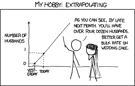
Think about this relationship in terms of causation.

Claim: Less sleep causes poorer daytime functioning.

Why might it be inappropriate to make the claim above based on these data alone? Think about what sort of study could provide stronger evidence for such a claim.

Things to think about:

• comparison groups.
  
• random allocation.
  
• measures of daytime functioning.
  
• measures of sleep time.
  
• other (unmeasured) explanatory variables.

Attendance and Attainment

Data: Education SIMD Indicators

The Scottish Government regularly collates data across a wide range of societal, geographic, and health indicators for every “datazone” (small area) in Scotland.

The dataset at https://uoepsy.github.io/data/simd20_educ.csv contains some of the education indicators (see Table 2).

Table 2: Education indicators from the 2020 SIMD data

variable	description
intermediate_zone	Areas of scotland containing populations of between 2.5k-6k household residents
attendance	Average School pupil attendance
attainment	Average attainment score of School leavers (based on Scottish Credit and Qualifications Framework (SCQF))
university	Proportion of 17-21 year olds entering university

Question 5

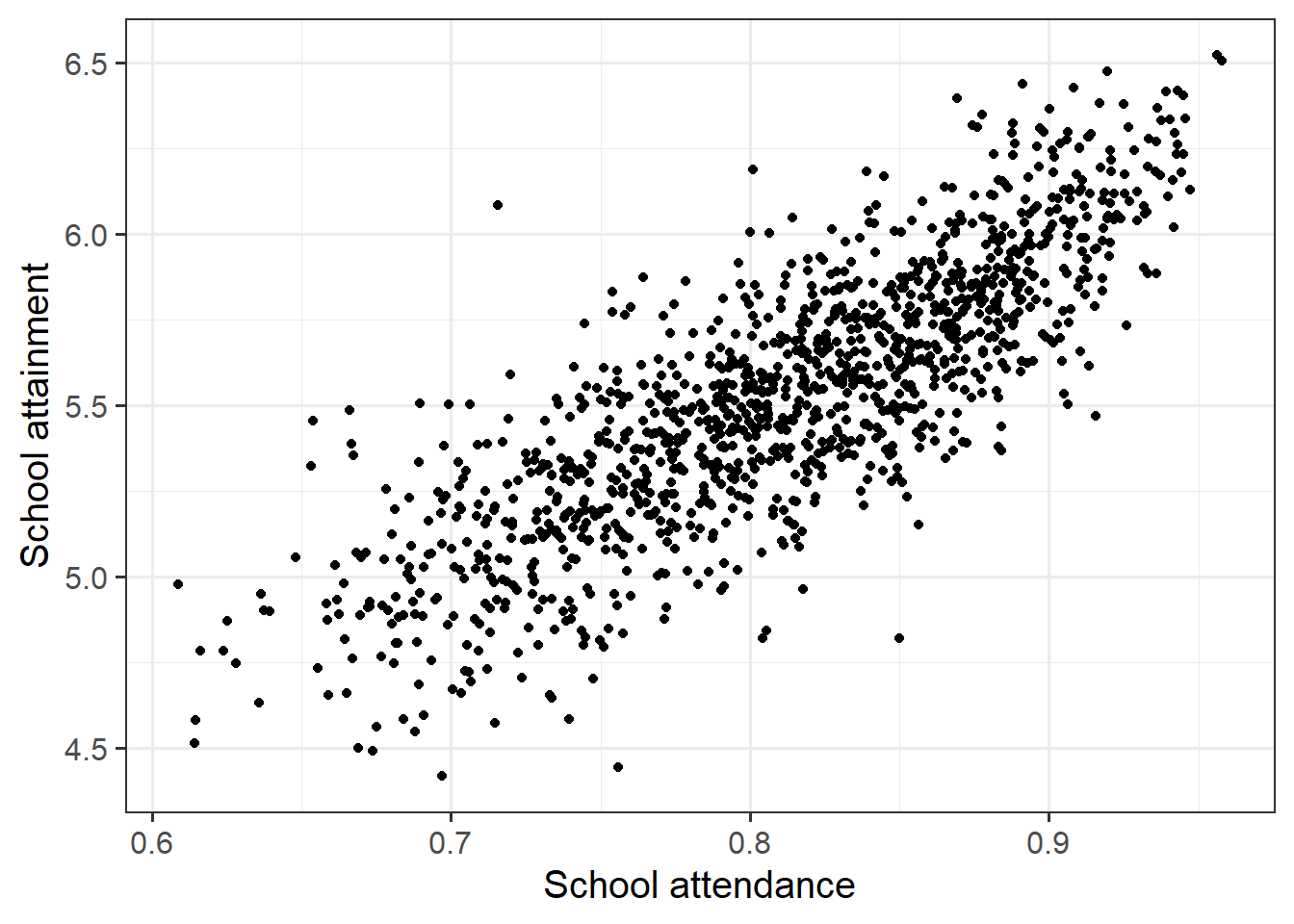
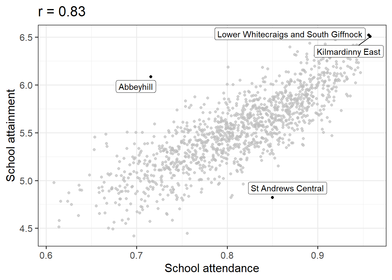
Conduct a test of whether there is a correlation between school attendance and school attainment in Scotland.

Present and write up the results.

Hints:

The readings have not included an example write-up for you to follow. Try to follow the logic of those for t-tests and \(\chi^2\)-tests.

• describe the relevant data
• explain what test was conducted and why
• present the relevant statistic, degrees of freedom (if applicable), statement on p-value, etc.
• state the conclusion.

Be careful figuring out how many observations your test is conducted on. cor.test() includes only the complete observations.

Solution

simd <- read_csv("https://uoepsy.github.io/data/simd20_educ.csv")

Here are the means of the two variables. We should remember that these calculations will include some observations which have missing data on the other variable.

simd %>% 
  summarise(
    m_attendance = mean(attendance, na.rm = TRUE),
    m_attainment = mean(attainment, na.rm = TRUE)
)

# A tibble: 1 × 2
  m_attendance m_attainment
         <dbl>        <dbl>
1        0.811         5.53

Instead, to match with out analysis, we might be inclined to filter our data to complete data:

simd_comp <- simd %>% 
  filter(!is.na(attendance) & !is.na(attainment))

simd_comp %>%
  summarise(
    m_attendance = mean(attendance),
    m_attainment = mean(attainment),
    sd_attendance = sd(attendance),
    sd_attainment = sd(attainment)
)

# A tibble: 1 × 4
  m_attendance m_attainment sd_attendance sd_attainment
         <dbl>        <dbl>         <dbl>         <dbl>
1        0.811         5.53        0.0696         0.386

cor.test(simd_comp$attendance, simd_comp$attainment)

    Pearson's product-moment correlation

data:  simd_comp$attendance and simd_comp$attainment
t = 51.495, df = 1242, p-value < 2.2e-16
alternative hypothesis: true correlation is not equal to 0
95 percent confidence interval:
 0.8066637 0.8421951
sample estimates:
      cor 
0.8252442 

A correlation test was conducted to assess whether there is a relationship between an area’s average school attendance, and its average school attainment level. A total of 1244 geographical areas were included in the analysis, with a mean school attendance of 0.81 (SD = 0.07) and a mean school attainment score of 5.53 (SD = 0.39).
There was a strong positive correlation between a geographical area’s level of school attendance and its school attainment (\(r\) = 0.83, \(t(1242\) = 51.5, \(p < 0.001\)). We therefore reject the null hypothesis that there is no correlation between an area’s school attendance and attainment. Figure 1 provides a visualisation of the relationship.

Code

ggplot(simd_comp, aes(x=attendance, y=attainment)) + 
  geom_point() + 
  labs(x = "School attendance",
       y = "School attainment")

Figure 1: Positive relationship between geographical areas’ level of school attendance and school attainment

Optional Optional: some extra plotting bits

Sometimes we may want to highlight certain parts of a plot. We can do that using the gghighlight package, and giving it a set of conditions (like we do for filter()) in order for it to decide which points to highlight.
You can see an example below.
We have also created the title by referring to the cor() function, and ’paste’ing it together to “r =”

library(gghighlight)

ggplot(simd_comp, aes(x=attendance, y=attainment)) + 
  geom_point() + 
  gghighlight( (attainment>6 & attendance<.75) | 
               attendance > .95 | 
               (attendance > .82 & attainment<5),
               label_key = intermediate_zone) + 
  labs(x = "School attendance",
       y = "School attainment",
       title = paste0("r = ",
                       round(
                         cor(simd_comp$attendance,
                                  simd_comp$attainment),
                         2)
                       ))

Functions and Models

Question 6

The Scottish National Gallery kindly provided us with measurements of side and perimeter (in metres) for a sample of 10 square paintings.

The data are provided below:
Note: this is a way of creating a “tibble” (a dataframe in ‘tidyverse-style’ language) in R, rather than reading one in from an external file.

sng <- tibble(
  side = c(1.3, 0.75, 2, 0.5, 0.3, 1.1, 2.3, 0.85, 1.1, 0.2),
  perimeter = c(5.2, 3.0, 8.0, 2.0, 1.2, 4.4, 9.2, 3.4, 4.4, 0.8)
)

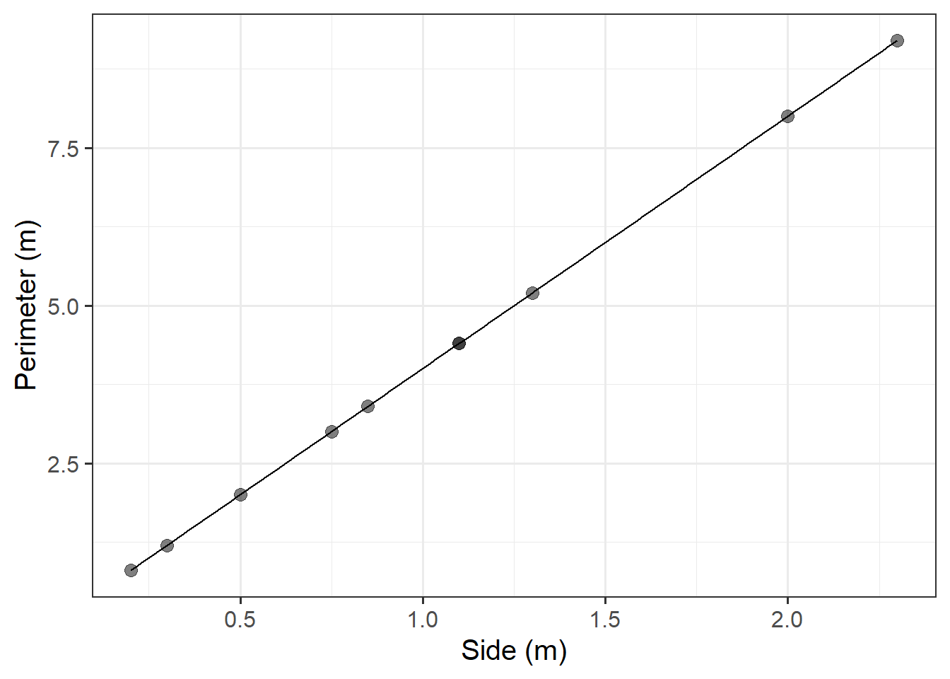
Plot the data from the Scottish National Gallery using ggplot(), with the side measurements of the paintings on the x-axis, and the perimeter measurements on the y-axis.

We know that there is a mathematical model for the relationship between the side-length and perimeter of squares: \(perimeter = 4 \times \ side\).

Try adding the following line to your plot:

  stat_function(fun = ~.x * 4)

Solution

sng <- tibble(
  side = c(1.3, 0.75, 2, 0.5, 0.3, 1.1, 2.3, 0.85, 1.1, 0.2),
  perimeter = c(5.2, 3.0, 8.0, 2.0, 1.2, 4.4, 9.2, 3.4, 4.4, 0.8)
)

ggplot(data = sng, aes(x = side, y = perimeter)) +
  geom_point(colour = 'black', alpha = 0.5, size = 3) +
  labs(x = 'Side (m)', y = 'Perimeter (m)')+
  stat_function(fun = ~.x * 4)

Figure 2: The exact relationship between side and perimeter of squares.

The above plot shows perfect agreement between the observed data and the model.

Question 7

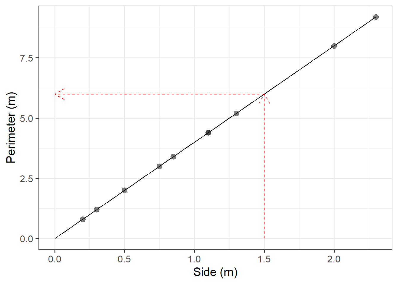
Use our mathematical model to predict the perimeter of a painting with a side of 1.5 metres.

Hints:
We don’t have a painting with a side of 1.5 metres within the random sample of paintings from the Scottish National Gallery, but we can work out the perimeter of an hypothetical square painting with 1.5m sides, using our model - either using the plot from the previous question, or calculating it algebraically.

Solution

Visual approach

Sometimes we can directly read a predicted value from the graph of the functional relationship.

Consider the plot created in the previous question. First, we need to check where x = 1.5. Then, we draw a vertical dashed line until it meets the blue line. The y value corresponding to x = 1.5 can be read off the y-axis.

However, in this case it is not that easy to read it from the drawing… Let’s try the next approach.

Algebraic approach

You can substitute the x value in the formula and calculate the corresponding y value.

\[ \begin{align} perimeter &= 4 \times \ side \\ &= 4 \times \ (1.5) \\ &= 6 \end{align} \]

The predicted perimeter of squared paintings having a 1.5m side is 6m.

NOTE: Don’t forget to always include the measurement units when reporting/writing-up results!

Data: HandHeight

This dataset, from Jessican M Utts and Robert F Heckard. 2015. Mind on Statistics (Cengage Learning)., records the height and handspan reported by a random sample of 167 students as part of a class survey.

The variables are:

• height, measured in inches
• handspan, measured in centimetres

The data are available at https://uoepsy.github.io/data/handheight.csv

Question 8

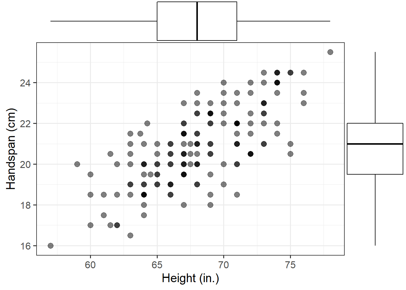
Consider the relationship between height (in inches) and handspan (in cm).

Read the handheight data into R, and investigate (visually) how handspan varies as a function of height for the students in the sample.

Do you notice any outliers or points that do not fit with the pattern in the rest of the data?

Comment on any main differences you notice between this relationship and the relationship between sides and perimeter of squares.

Solution

The handheight data set contains two variables, height and handspan, which are both numeric and continuous. We display the relationship between two numeric variables with a scatterplot.

We can also add marginal boxplots for each variable using the package ggExtra. Before using the package, make sure you have it installed via install.packages('ggExtra').

handheight <- read_csv(file = 'https://uoepsy.github.io/data/handheight.csv')

library(ggExtra)

plt <- ggplot(handheight, aes(x = height, y = handspan)) +
  geom_point(size = 3, alpha = 0.5) +
  labs(x = 'Height (in.)', y = 'Handspan (cm)')

ggMarginal(plt, type = 'boxplot')

Figure 3: The statistical relationship between height and handspan.

Outliers are extreme observations that do not seem to fit with the rest of the data. This could either be:

• marginally along one axis: points that have an unusual (too high or too low) x-coordinate or y-coordinate;
• jointly: observations that do not fit with the rest of the point cloud.

The boxplots in fig-handheight-scatterplot do not highlight any outliers in the marginal distributions of height and handspan. Furthermore, from the scatterplot we do not notice any extreme observations or points that do not fit with the rest of the point cloud.

We notice a moderate, positive (that is, increasing) linear relationship between height and handspan.

Recall Figure 2, displaying the relationship between side and perimeters of squares. In the plot we notice two points on top of each other, reflecting the fact that two squares having the same side will always have the same perimeter. In fact, the data from the Scottish National Gallery include two squared paintings with a side of 1.1m, both having a measured perimeter of 4.4m.

fig-handheight-scatterplot, instead, displays the relationship between height and handspan of a sample of students. The first thing that grabs our attention is the fact that students having the same height do not necessarily have the same handspan. Rather, we clearly see a variety of handspan values for students all having a height of, for example, 70in. To be more precise, the seven students who are 70 in. tall all have differing handspans.

Question 9

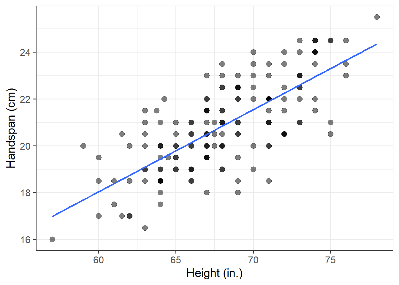
Hopefully, as part of the previous question, you created a scatterplot of handspans against heights. If not, make one now.

Try adding the following line of code to the scatterplot. It will add a best-fit line describing how handspan varies as a function of height. For the moment, the argument se = FALSE tells R to not display uncertainty bands.

geom_smooth(method = lm, se = FALSE)

Think about the differences you notice with between this and the figure you made in Question 6.

Solution

ggplot(handheight, aes(x = height, y = handspan)) +
  geom_point(size = 3, alpha = 0.5) +
  geom_smooth(method = lm, se = FALSE) +
  labs(x = 'Height (in.)', y = 'Handspan (cm)')

Figure 4: The best-fit line.

The line representing the relationship between side and perimeter of squares (Figure 2) is able to predict the actual perimeter value from the measurement of the side of a square. This is possible because the relationship between side and perimeter is an exact one. That is, any squares having the same side will have the same perimeter, and there will be no variation in those values.

The line that best fits the relationship between height and handspan (Figure 4) is only able to predict the average handspan for a given value of height. This is because there will be a distribution of handspans at each value of height. The line will fit the trend/pattern in the values, but there will be individual-to-individual variability that we must accept around that average pattern.

Relationships such as that between height and handspan show deviations from an “average pattern”. To model this, we need need to create a model that allows for deviations from the linear relationship. This is called a statistical model.

A statistical model includes both a deterministic function and a random error term:

\[ Handspan = \beta_0 + \beta_1 \ Height + \epsilon \]

or, in short,

\[ y = \underbrace{\beta_0 + \beta_1 \ x}_{f(x)} + \underbrace{\epsilon}_{\text{random error}} \]

The deterministic function \(f(x)\) need not be linear if the scatterplot displays signs of nonlinearity, but in this course we focus primarily on linear relationships.

In the equation above, the terms \(\beta_0\) and \(\beta_1\) are numbers specifying where the line going through the data meets the y-axis and its slope (rate of increase/decrease).

Question 10

The line of best-fit is given by:¹

\[ \widehat{Handspan} = -3 + 0.35 \ Height \]

What is your best guess for the handspan of a student who is 73in tall?

And for students who are 5in?

Solution

The predicted average handspan for students who are 73in tall is \(-3 + 0.35 * 73 = 22.55\)cm.

The predicted average handspan for students who are 5in tall is \(-3 + 0.35 * 5 = -1.25\)cm. But wait, handspan can not be negative… This does not make any sense! That’s right, we went too far off the range of the available data on heights, which were between 57in and 78in. We extrapolated. This is very dangerous…

Figure 5: Source: Randall Munroe, xkcd.com

Footnotes

1. Yes, the error term is gone. This is because the line of best-fit gives you the prediction of the average handspan for a given height, and not the individual handspan of a person, which will almost surely be different from the prediction of the line.