Week 3 Exercises: T-tests

Procrastination Scores

Research Question Do Edinburgh University students report endorsing procrastination less than the norm?

The Procrastination Assessment Scale for Students (PASS) was designed to assess how individuals approach decision situations, specifically the tendency of individuals to postpone decisions (see Solomon & Rothblum, 1984). The PASS assesses the prevalence of procrastination in six areas: writing a paper; studying for an exam; keeping up with reading; administrative tasks; attending meetings; and performing general tasks. For a measure of total endorsement of procrastination, responses to 18 questions (each measured on a 1-5 scale) are summed together, providing a single score for each participant (range 0 to 90). The mean score from Solomon & Rothblum, 1984 was 33.

A student administers the PASS to 20 students from Edinburgh University.
The data are available at https://uoepsy.github.io/data/pass_scores.csv.

Question 1

1. Read in the data
2. Calculate some relevant descriptive statistics
3. Check the assumptions that we will be concerned with for a one-sample test of whether the mean PASS scores is less than 33.

Solution

Read in the data:

pass_scores <- read_csv("https://uoepsy.github.io/data/pass_scores.csv") 

Descriptives:

pass_scores %>%
  summarise(
    mPASS = mean(PASS),
    sdPASS = sd(PASS)
  )

# A tibble: 1 × 2
  mPASS sdPASS
  <dbl>  <dbl>
1  30.7   3.31

Assumptions:

We want to check that the data are close to normally distributed. This is especially relevant as we have only 20 datapoints here. The plot below makes it look like we may have one or two data points in the tails of the distribution that are further than we might expect.

ggplot(pass_scores, aes(sample = PASS)) + 
  geom_qq() + 
  geom_qq_line()

But the Shapiro-Wilk test of \(p > .05\) indicates that we are probably okay to continue with our t-test

shapiro.test(pass_scores$PASS)

    Shapiro-Wilk normality test

data:  pass_scores$PASS
W = 0.93617, p-value = 0.2028

Question 2

Our test here is going to be have the following hypotheses:

• Null: mean PASS score in Edinburgh Uni students is \(\geq 33\)
• Alternative: mean PASS score in Edinburgh Uni students is \(< 33\)

Read in the data and manually calculate the relevant test statistic.
Note, we’re doing this manually right now as it’s a useful learning process. In later questions we will switch to the easy way!

Hints:

• you can see the manual calculation of a one sample t-test in 3B #one-sample-t-test.
• The relevant formula is:

\[ \begin{align} & t = \frac{\bar x - \mu_0}{\frac{s}{\sqrt{n}}} \\ \qquad \\ & \text{Where:} \\ & \bar x : \text{mean of PASS in our sample} \\ & \mu_0 : \text{hypothesised mean score of 33} \\ & s : \text{standard deviation of PASS in our sample} \\ & n : \text{number of observations} \end{align} \]

Solution

pass_scores <- read_csv("https://uoepsy.github.io/data/pass_scores.csv") 

pass_scores %>% 
  summarise(
    xbar = mean(PASS),
    s = sd(PASS),
    n = n(),
    t = (xbar - 33)/(s / sqrt(n))
  )

# A tibble: 1 × 4
   xbar     s     n     t
  <dbl> <dbl> <int> <dbl>
1  30.7  3.31    20 -3.11

Question 3

Using the test statistic calculated in question 1, compute the p-value.

Hint:

• this will be needing the pt() function.
• the degrees of freedom is \(n-1\) (we used one up by estimating the mean).
• The test we are performing is against the null hypothesis that the mean is \(\geq 33\). Our t-statistic is in the broad sense calculated as “mean minus 33”, so negative numbers mean we have a mean lower than 33. These are the instances that we will reject the null hypothesis - if we get a test statistic very low. So we want the lower.tail of the distribution for our p-value.

Solution

We have 20 participants, so \(df=19\)

pt(-3.107272, df = 19, lower.tail = TRUE)

[1] 0.002900159

Question 4

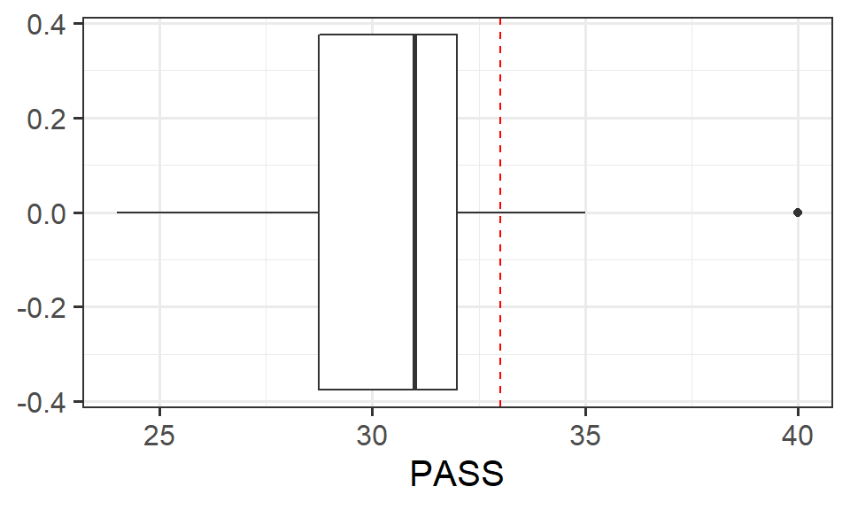
Now using the t.test() function, conduct the same test. Check that the numbers match with questions 1 and 2, and create a visualisation to illustrate any results.

Hint: Check out the help page for t.test() - there is an argument in the function that allows us to easily change between whether our alternative hypothesis is “less than”, “greater than” or “not equal to”.

Solution

t.test(pass_scores$PASS, mu = 33, alternative = "less")

    One Sample t-test

data:  pass_scores$PASS
t = -3.1073, df = 19, p-value = 0.0029
alternative hypothesis: true mean is less than 33
95 percent confidence interval:
    -Inf 31.9799
sample estimates:
mean of x 
     30.7 

ggplot(data = pass_scores, aes(x=PASS)) + 
  geom_boxplot() + 
  geom_vline(xintercept=33, lty="dashed", col="red")

Question 5

Write up the results.

Hints: There are some quick example write-ups for each test in 3B #basic-tests

Solution

A one-sided one-sample t-test was conducted in order to determine if the average score on the Procrastination Assessment Scale for Students (PASS) for a sample of 20 students at Edinburgh University was significantly lower (\(\alpha = .05\)) than the average score obtained during development of the PASS.

Edinburgh University students scored lower (Mean = 30.7, SD = 3.31) than the score reported by the authors of the PASS (Mean = 33). This difference was statistically significant (t(19)=-3.11, p < .05, one-tailed).

Heights

Research Question Is the average height of students taking the USMR statistic course in Psychology at Edinburgh University in 2021/2022 is different from 165cm?

The data for students from all psychology statistics courses last year and USMR this year, are available at https://uoepsy.github.io/data/surveydata_allcourse22.csv.

Question 6

No more manual calculations of test statistics and p-values for this week.

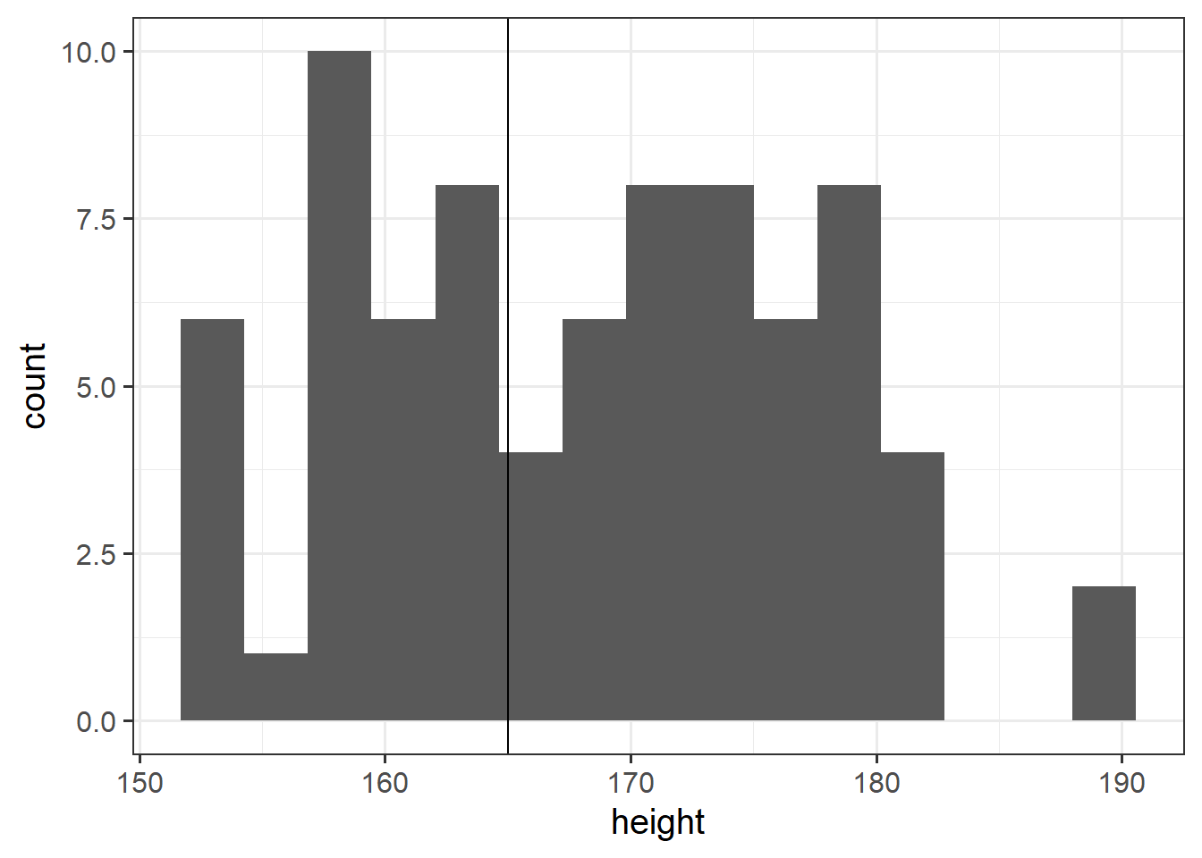
Conduct a one sample \(t\)-test to evaluate whether the average height of students taking the USMR courses in Psychology at Edinburgh University in 2022/23 is different from 165cm.

Hints:

• This is real data, and real data is rarely normal! If you conduct a Shapiro-Wilk test, you may well find \(p<.05\) and conclude that your data is not normal.
  So what do we do if a test indicates our assumptions are violated?
  Well, we should bear a couple of things in mind.
  1. A decision rule such as \(p<.05\) on Shapiro-Wilk test creates very dichotomous thinking for something which is in reality not black and white. Real life distributions are not either normal or non-normal. Plot the data, and make a judgement!
     
  2. As it happens, the t-test is actually reasonably robust against slight deviations from normality! Plot your data and make a judgement!
  3. The deeper you get into statistics, the more you discover that it is not simply a case of following step-by-step rules:

Solution

Read in the data:

We need to filter it to just the USMR students this year

survey_data <- read_csv("https://uoepsy.github.io/data/surveydata_allcourse22.csv")

usmr_data <- survey_data %>% 
  filter(course=="usmr", year==2022)

Descriptives:

usmr_data %>% 
  summarise(
    mheight = mean(height, na.rm = T),
    sdheight = sd(height, na.rm = T)
  )

# A tibble: 1 × 2
  mheight sdheight
    <dbl>    <dbl>
1    168.     9.10

Assumptions:

The shapiro.test() suggests that our assumption of normality is not okay!
(the p-value is \(<.05\), suggesting that we reject the hypothesis that the data are drawn from a normally distributed population)

shapiro.test(usmr_data$height)

    Shapiro-Wilk normality test

data:  usmr_data$height
W = 0.96802, p-value = 0.0494

However, as always, visualisations are vital here. The histogram below doesn’t look all that great, but the t.test is quite robust against slight violations of normality, especially as sample sizes increase beyond 30, and our data here doesn’t look too non-normal (this is a judgement call here - over time you will start to get a sense of what you might deem worrisome in these plots!).

ggplot(data = usmr_data, aes(x = height)) + 
  geom_histogram(bins=15) +
  # adding our hypothesised mean
  geom_vline(xintercept = 165) 

Conduct test

t.test(usmr_data$height, mu = 165, alternative = "two.sided")

    One Sample t-test

data:  usmr_data$height
t = 2.9983, df = 76, p-value = 0.003667
alternative hypothesis: true mean is not equal to 165
95 percent confidence interval:
 166.0442 170.1761
sample estimates:
mean of x 
 168.1101 

Names and Tips

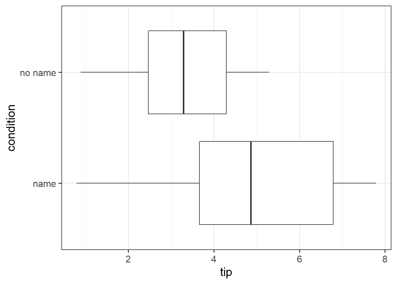
Research Question Can a server earn higher tips simply by introducing themselves by name when greeting customers?

Researchers investigated the effect of a server introducing herself by name on restaurant tipping. The study involved forty, 2-person parties eating a $23.21 fixed-price buffet Sunday brunch at Charley Brown’s Restaurant in Huntington Beach, California, on April 10 and 17, 1988. Each two-person party was randomly assigned by the waitress to either a name or a no name introduction condition using a random mechanism. The waitress kept track of the two-person party condition and how much the party paid at the end of the meal.

The data are available at https://uoepsy.github.io/data/gerritysim.csv. (This is a simulated example based on Garrity and Degelman (1990))

Question 7

Conduct an independent samples \(t\)-test to assess whether higher tips are earned when the server introduces themselves by name, in comparison to when they do not.

Hints:

• We’ll want to check the normality (either visually or with a test) of the variable of interest for each group.
  
• Some researchers suggest using the Welch t-test by default. This means you can relax the assumption of equal variances in the groups. If you want to test whether two variances are equal, try the var.test() function.

Solution

Read in the data

tipdata <- read_csv("https://uoepsy.github.io/data/gerritysim.csv")

#make a "tip" column, which is minus the meal amount
tipdata <- 
  tipdata %>% mutate(
    tip = paid - 23.21
  )

Descriptives and a plot

tipdata %>% 
  group_by(condition) %>%
  summarise(
    meantip = mean(tip),
    sdtip = sd(tip)
  )

# A tibble: 2 × 3
  condition meantip sdtip
  <chr>       <dbl> <dbl>
1 name         4.94  1.88
2 no name      3.18  1.35

ggplot(data = tipdata, aes(x = tip, y = condition)) +
  geom_boxplot()

Assumptions

According to these tests, we have normally distributed data for both groups, with equal variances.

shapiro.test(tipdata$tip[tipdata$condition=="name"])

    Shapiro-Wilk normality test

data:  tipdata$tip[tipdata$condition == "name"]
W = 0.96267, p-value = 0.5985

shapiro.test(tipdata$tip[tipdata$condition=="no name"])

    Shapiro-Wilk normality test

data:  tipdata$tip[tipdata$condition == "no name"]
W = 0.94405, p-value = 0.2857

var.test(tip ~ condition, data = tipdata)

    F test to compare two variances

data:  tip by condition
F = 1.9344, num df = 19, denom df = 19, p-value = 0.1595
alternative hypothesis: true ratio of variances is not equal to 1
95 percent confidence interval:
 0.7656473 4.8870918
sample estimates:
ratio of variances 
           1.93437 

Conduct test:

Because the variances do not appear to be unequal, we can actually use the standard t-test with var.equal = TRUE if we want. However, we’ll continue with the Welch t-test.

Remember that our alternative hypothesis here is that the average tips in the “name” condition is greater than in the “no name” condition.
R will take the levels in order here (alphabetically), and assume that the alternative is for that group, so we use alternative = "greater" here to say that the alternative is \(\text{name}-\text{no name} > 0\).

t.test(tip ~ condition, data = tipdata, alternative = "greater")

    Welch Two Sample t-test

data:  tip by condition
t = 3.4117, df = 34.502, p-value = 0.0008314
alternative hypothesis: true difference in means between group name and group no name is greater than 0
95 percent confidence interval:
 0.8893105       Inf
sample estimates:
   mean in group name mean in group no name 
               4.9450                3.1825 

Optional Extras

Question Extra

Here are a few extra questions for you to practice performing tests and making plots:

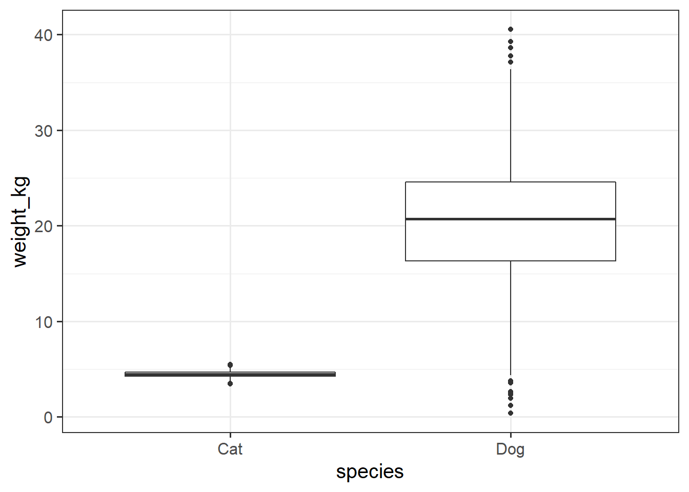
1. Are dogs heavier on average than cats?

• Data are at https://uoepsy.github.io/data/pets_seattle.csv
  
• Remember from week 1 - not everything in that data is either a cat or a dog!

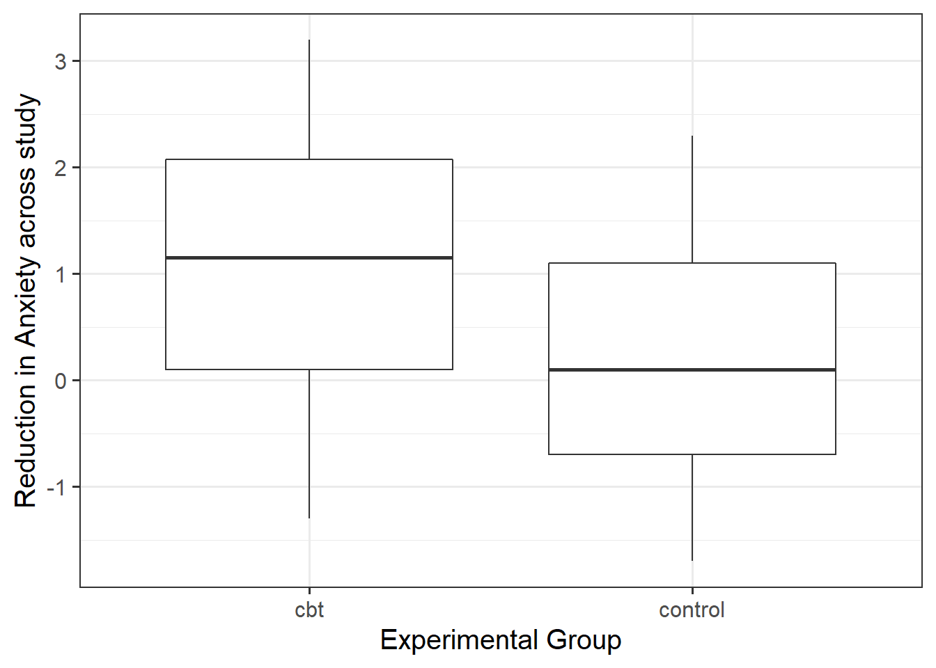
2. Is taking part in a cognitive behavioural therapy (CBT) based programme associated with a greater reduction, on average, in anxiety scores in comparison to a Control group?

• Data are at https://uoepsy.github.io/data/dapr1_2122_report_data.csv. The dataset contains information on each person in an organisation, recording their professional role (management vs employee), whether they are allocated into the CBT programme or not (control vs cbt), and scores on anxiety at both the start and the end of the study period.
  • you might have to make a new variable in order to test the research question.

Solution

Cats v Dogs

pets <- read.csv("https://uoepsy.github.io/data/pets_seattle.csv")
catsndogs <- pets[pets$species != "Goat", ]

In this case, we want to test whether \(dogs > cats\). What we are testing then, whether \(dogs - cats > 0\) or \(cats - dogs < 0\).
By default, as the species variable is a character, it will use alphabetical ordering, and t.test() will test \(cats - dogs\). So we want our alternative hypothesis to be “less”:

t.test(weight_kg ~ species, catsndogs,
       alternative = "less")

An alternative is to set it as a factor, and specify the levels in the order we want:

catsndogs$species2 <- factor(catsndogs$species, levels = c("Dog","Cat"))

Which would then allow us to shove that into the t.test() and perform the same test, but using \(dogs - cats\) instead.

t.test(weight_kg ~ species2, catsndogs,
       alternative = "greater")

    Welch Two Sample t-test

data:  weight_kg by species2
t = 92.4, df = 1335.2, p-value < 2.2e-16
alternative hypothesis: true difference in means between group Dog and group Cat is greater than 0
95 percent confidence interval:
 15.60965      Inf
sample estimates:
mean in group Dog mean in group Cat 
        20.377489          4.484731 

catsndogs %>%
  ggplot(aes(x=species,y=weight_kg)) + 
  geom_boxplot()

CBT & Anxiety

Because we’re testing the reduction in anxiety, we need to calculate it. By subtracting anxiety at time 2 from anxiety at time 1, we create a variable for which bigger values represent more reduction in anxiety

cbtanx <- read.csv("https://uoepsy.github.io/data/dapr1_2122_report_data.csv")

cbtanx <- cbtanx %>% mutate(reduction = anx_t1 - anx_t2)

And we can then test whether \(cbt - control > 0\):

t.test(reduction ~ cbt, data = cbtanx, 
       alternative = "greater")

    Welch Two Sample t-test

data:  reduction by cbt
t = 2.5953, df = 56.621, p-value = 0.006007
alternative hypothesis: true difference in means between group cbt and group control is greater than 0
95 percent confidence interval:
 0.2744051       Inf
sample estimates:
    mean in group cbt mean in group control 
            1.0266667             0.2551724 

And to make sure we’re getting things the right way around, make a plot:

ggplot(cbtanx, aes(x=cbt, y=reduction))+
  geom_boxplot() + 
  labs(x="Experimental Group",y="Reduction in Anxiety across study")