Exercises: GLM

Question 1

Before doing anything else, watch this video, and try to count exactly how many times the players wearing white pass the basketball.

Invisible Gorillas

Data: invisibleg.csv

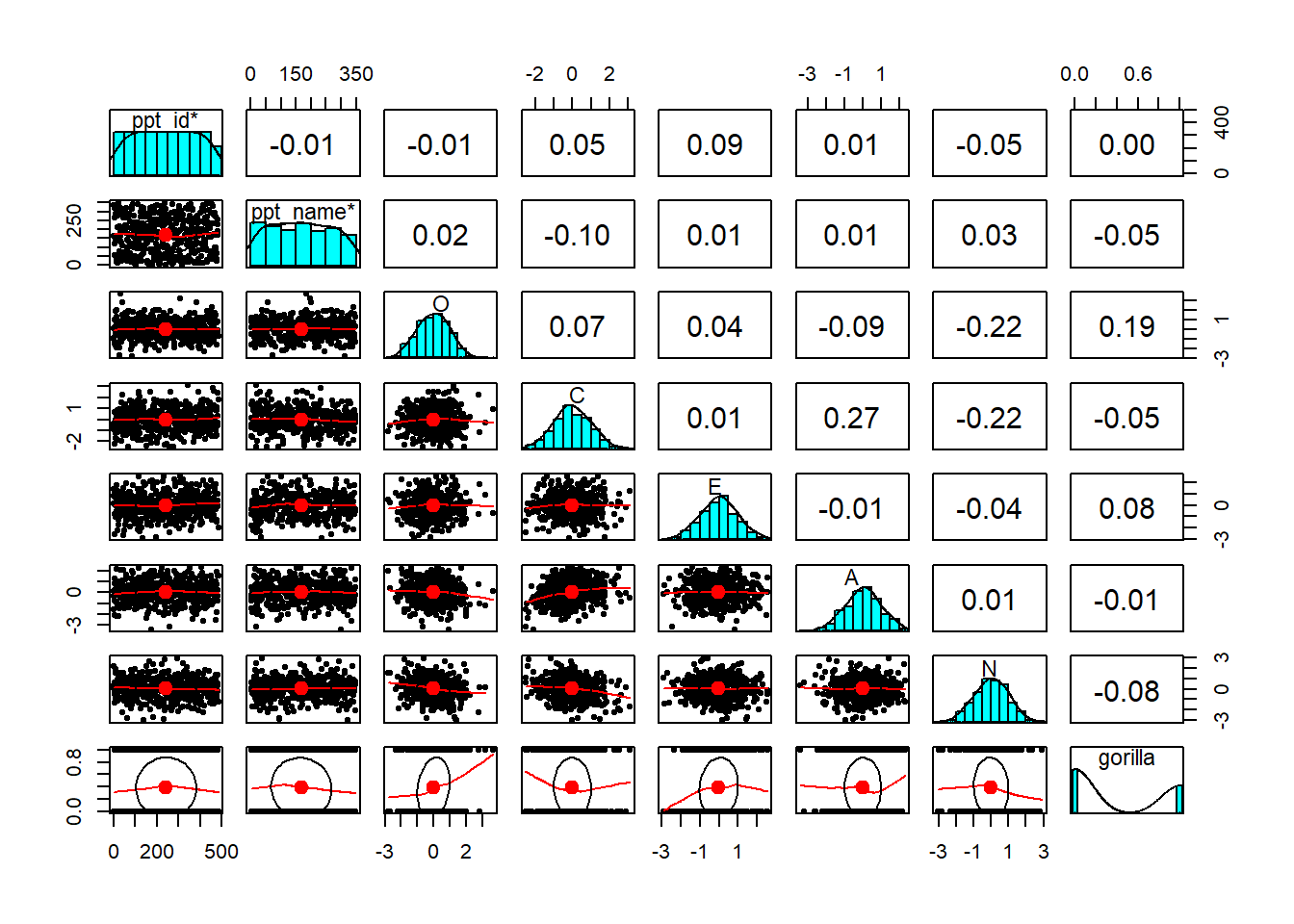
The data here come from a study of 483 participants who completed a Big 5 Personality Inventory (providing standardised scores on 5 personality traits of Openness, Conscientiousness, Extraversion, Agreeableness and Neuroticism), and then completed the selective attention task as seen above, from Simons & Chabris 1999.

We’re interested in whether and how individual differences in personality are associated with susceptibility to inattentional blindness (i.e. not noticing the gorilla).

The data are available at https://uoepsy.github.io/data/invisibleg.csv.

Table 1:

Data dictionary for invisibleg.csv

variable	description
ppt_id	Participant ID number
ppt_name	Participant Name (if recorded)
O	Openness (Z-scored)
C	Conscientiousness (Z-scored)
E	Extraversion (Z-scored)
A	Agreeableness (Z-scored)
N	Neuroticism (Z-scored)
gorilla	Whether or not participants noticed the gorilla (0 = did not notice, 1 = did notice)

Question 2

Read in the data, have a look around, plot, describe, and generally explore.
Do any cleaning that you think might be necessary.

Hints

There’s nothing new to any of the data cleaning that needs done here. We can do everything that needs doing by using something like ifelse().

invis <- read_csv("https://uoepsy.github.io/data/invisibleg.csv")

summary(invis)

    ppt_id            ppt_name               O                   C            
 Length:483         Length:483         Min.   :-2.786578   Min.   :-2.510626  
 Class :character   Class :character   1st Qu.:-0.687997   1st Qu.:-0.659786  
 Mode  :character   Mode  :character   Median : 0.011968   Median :-0.030208  
                                       Mean   :-0.001907   Mean   : 0.005702  
                                       3rd Qu.: 0.685956   3rd Qu.: 0.675251  
                                       Max.   : 3.667985   Max.   : 3.119541  
       E                   A                  N                gorilla        
 Min.   :-2.916437   Min.   :-3.39605   Min.   :-99.00000   Min.   :-99.0000  
 1st Qu.:-0.678922   1st Qu.:-0.63624   1st Qu.: -0.66889   1st Qu.:  0.0000  
 Median : 0.012801   Median : 0.03289   Median :  0.01216   Median :  0.0000  
 Mean   :-0.008537   Mean   : 0.01091   Mean   : -0.81698   Mean   : -0.8468  
 3rd Qu.: 0.693415   3rd Qu.: 0.66549   3rd Qu.:  0.71102   3rd Qu.:  1.0000  
 Max.   : 2.544318   Max.   : 2.31373   Max.   :  2.94009   Max.   :  1.0000  

Right away we can see there’s something odd with the Neuroticism variable (N). It shouldn’t have values of -99.

As it happens, a well-known statistical software package (ahem) often ends with missing values being stored as “-99”, or “-999”.

We can also see that we have some “-99” in the gorilla variable.

So let’s replace all those with NA’s

invis <- invis |>
  mutate(
    N = ifelse(N == -99, NA, N),
    gorilla = ifelse(gorilla == -99, NA, gorilla)
  )

summary(invis)

    ppt_id            ppt_name               O                   C            
 Length:483         Length:483         Min.   :-2.786578   Min.   :-2.510626  
 Class :character   Class :character   1st Qu.:-0.687997   1st Qu.:-0.659786  
 Mode  :character   Mode  :character   Median : 0.011968   Median :-0.030208  
                                       Mean   :-0.001907   Mean   : 0.005702  
                                       3rd Qu.: 0.685956   3rd Qu.: 0.675251  
                                       Max.   : 3.667985   Max.   : 3.119541  
                                                                              
       E                   A                  N                gorilla      
 Min.   :-2.916437   Min.   :-3.39605   Min.   :-3.057349   Min.   :0.0000  
 1st Qu.:-0.678922   1st Qu.:-0.63624   1st Qu.:-0.630916   1st Qu.:0.0000  
 Median : 0.012801   Median : 0.03289   Median : 0.016932   Median :0.0000  
 Mean   :-0.008537   Mean   : 0.01091   Mean   : 0.002915   Mean   :0.3878  
 3rd Qu.: 0.693415   3rd Qu.: 0.66549   3rd Qu.: 0.724583   3rd Qu.:1.0000  
 Max.   : 2.544318   Max.   : 2.31373   Max.   : 2.940095   Max.   :1.0000  
                                        NA's   :4           NA's   :6       

There’s not a great deal to describe here, because our variables are already Z-scored (i.e. they all have means of 0 and standard deviations of 1).

It’s still important to look at our data though:

psych::pairs.panels(invis)

And we can tabulate the number of participants that do/don’t notice the gorilla:

table(invis$gorilla)

  0   1 
292 185 

Only 39% of people noticed the gorilla!

Question 3

Here is an “intercept-only” model of the binary outcome ‘did they notice the gorilla or not’:

glm(gorilla ~ 1, data = invis, family=binomial) |>
  summary()

...
Coefficients:
            Estimate Std. Error z value Pr(>|z|)    
(Intercept) -0.45640    0.09397  -4.857 1.19e-06 ***

1. Convert the intercept estimate from log-odds into odds
   
2. Convert those odds into probability
   
3. What does that probability represent?
   • hint: in lm(y~1) the intercept is the same as mean(y)

The intercept estimate of -0.456 is in log-odds.

To convert from log-odds to odds, we exponentiate (\(odds = e^{log-odds}\))

The odds of noticing the gorilla are \(e^{-0.456} = 0.634\).

To convert this back to probability, we calculate \(\frac{odds}{1+odds}\).

\(\frac{0.634}{1.634} = 0.388\).

So there is a 0.388 probability of a participant noticing the gorilla.

Does this number seem familiar?
Because there’s no predictors in the model, our intercept is just the proportion of 1s in our outcome variable!

prop.table(table(invis$gorilla))

        0         1 
0.6121593 0.3878407 

Question 4

Does personality (i.e. all our measured personality traits collectively) predict inattentional blindness?

Hints

We’re wanting to test the influence of a set of predictors here. Sounds like a job for model comparison! (see 10A #comparing-models).

BUT WAIT… we might have some missing data…
(this depends on whether, during your data cleaning, you a) replaced values of -99 with NA, or b) removed those entire rows from the data).

Models like lm() and glm() will exclude any observation (the entire row) if it has a missing value for any variable in the model (outcome or predictor). As we have missing data on the N variable, then when we put that in as a predictor, those rows are omitted from the model.

So we’ll need to ensure that both models that we are comparing are fitted to exactly the same set of observations.

If we just try a comparison, we get an error:

m0 <- glm(gorilla ~ 1, data = invis, family=binomial)
m1 <- glm(gorilla ~ O+C+E+A+N, data = invis, family=binomial)
anova(m0,m1, test="Chisq")

Error in anova.glmlist(c(list(object), dotargs), dispersion = dispersion, :
models were not all fitted to the same size of dataset

So what we need to do is fit both models to the data that has values for all of the variables in our full model.

If you haven’t discovered it already, na.omit(dataset) is a quick way to remove all rows that have incomplete data.

But we need to be careful - if we just use na.omit() on the entire dataset, then we could be removing a whole load of data that is actually perfectly useful to us:

# number of rows in entire dataset:
invis |> nrow()
# number of rows with complete data:
na.omit(invis) |> nrow()
# number of rows with complete data in the variables we're using in model:
na.omit(invis[,3:8]) |> nrow()

[1] 483
[1] 411
[1] 473

We can see that if we just used na.omit(invis) here, we would be removing 72 people. As it happens, this is excluding a whole bunch of participants for whom their names are missing. But we’re not using their names, so we can actually use these in our model!

moddat <- na.omit(invis[,3:8])

m0 <- glm(gorilla ~ 1, data = moddat,
          family=binomial)
m1 <- glm(gorilla ~ O+C+E+A+N, data = moddat, 
          family=binomial)

anova(m0,m1, test="Chisq")

Analysis of Deviance Table

Model 1: gorilla ~ 1
Model 2: gorilla ~ O + C + E + A + N
  Resid. Df Resid. Dev Df Deviance  Pr(>Chi)    
1       472     631.30                          
2       467     608.23  5   23.067 0.0003278 ***
---
Signif. codes:  0 '***' 0.001 '**' 0.01 '*' 0.05 '.' 0.1 ' ' 1

The inclusion of the Big 5 Personality Traits (Openness, Conscientiousness, Extraversion, Agreeablenss and Neuroticism) were found to result in a significant improvement in model fit over the null model (\(\chi^2(5)=23.07, p<0.001\)), suggesting that personality is useful in predicting inattentional blindness.

Question 5

How are different aspects of personality associated with inattentional blindness?

Hints

The interpretation of logistic regression coefficients is explained in 10A #coefficient-interpretation.

You might want to explain the key finding(s) in terms of odds ratios.

The coefficients we get from our model are in log-odds. So values \(<0\) represent decreasing probability, and values \(>0\) represent increasing probability.

But that’s about as much as we can interpret in this scale.
When we exponentiate them, we get our odds-ratios. These are “how much the odds are multiplied by”, so values \(<1\) represent decreased odds (i.e. decreasing probability) and values \(>1\) represent increased odds.

Only Openness (O) is significantly associated with the probability of noticing the gorilla.

coefficient	b	exp(b)	interpretation
(Intercept)	-0.48***	0.62***	for someone at the mean on all personality traits, the odds of noticing the gorilla are 0.62 to 1
O	0.38***	1.46***	holding other personality traits constant, being 1 SD higher on openness is associated with 1.46 times the odds of noticing the gorilla
C	-0.19	0.82
E	0.17	1.18
A	0.07	1.07
N	-0.13	0.88

Question 6

Compute confidence intervals for your odds ratios.

confidence interval refresher

We haven’t been using confidence intervals very much, but we very easily could have been. Functions like t.test(), cor.test() etc present confidence intervals in their output, and functions like confint() can be used on linear regression models to get confidence intervals for our coefficients.

Confidence intervals (CIs) are often used to make a statement about a null hypothesis just like a p-value (see 3A #inference. If a 95% CI does not contain zero then we can, with that same level of confidence, reject the null hypothesis that the population value is zero. So a 95% confidence interval maps to \(p<.05\), and a 99% CI maps to \(p<.01\), and so on.

However, many people these days prefer confidence intervals to \(p\)-values as they take the focus (slightly) away from the null hypothesis and toward a range of effect sizes that are compatible with the data.

The function confint() will give you confidence intervals. The function car::Confint()¹ will do exactly the same but put them alongside the estimates (which saves you scrolling up and down between different outputs).

exp(car::Confint(m1))

             Estimate     2.5 %    97.5 %
(Intercept) 0.6174089 0.5093876 0.7459179
O           1.4572206 1.1922054 1.7917164
C           0.8244801 0.6719649 1.0086947
E           1.1830867 0.9777058 1.4362320
A           1.0712494 0.8782219 1.3084848
N           0.8785279 0.7189474 1.0716537

holding other personality traits constant, being 1 SD higher on openness is associated with 1.46 (95% CI: 1.19, 1.79) times the odds of noticing the gorilla

Question 7

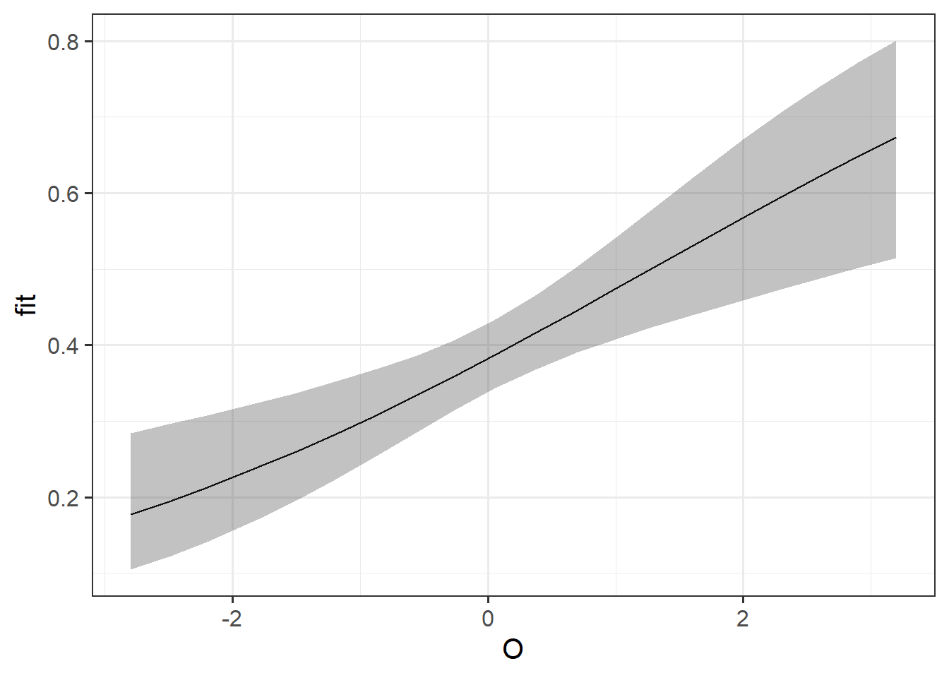
Produce a plot of the predicted probabilities of noticing the gorilla as a function of openness.

Hints

There’s an example of this at 10A #visualising. Using the effects package will be handy.

the xlevels argument here says to give us the fitted values for 20 different values across the predictor

library(effects)

effect(term = "O", mod = m1, xlevels = 20) |>
  as.data.frame() |>
  ggplot(aes(x=O,y=fit,ymin=lower,ymax=upper))+
  geom_line()+
  geom_ribbon(alpha=.3)

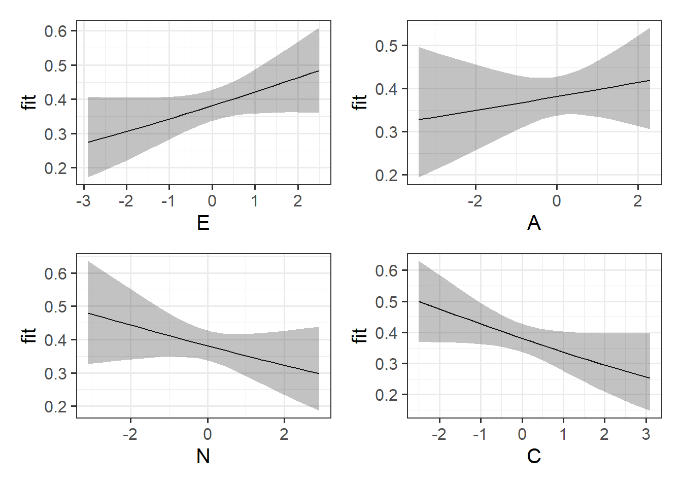
Question 8

Try creating an equivalent plot for the other personality traits - before you do, what do you expect them to look like?

From our coefficients, we should expect the lines to go up as E and A increase, and down as C and N increase.
However, for all of these, we should expect a lot of uncertainty (i.e. for all of these, 0 is inside our confidence intervals (i.e. they’re non-significant))

car::Confint(m1)

               Estimate       2.5 %       97.5 %
(Intercept) -0.48222369 -0.67454599 -0.293139778
O            0.37653095  0.17580488  0.583174041
C           -0.19300227 -0.39754917  0.008657158
E            0.16812690 -0.02254645  0.362022998
A            0.06882561 -0.12985594  0.268869789
N           -0.12950767 -0.32996703  0.069202969

e.g., for extraversion:

Code

library(patchwork)
plte <- effect(term = "E", mod = m1, xlevels = 20) |>
  as.data.frame() |>
  ggplot(aes(x=E,y=fit,ymin=lower,ymax=upper))+
  geom_line()+
  geom_ribbon(alpha=.3)

pltc <- effect(term = "C", mod = m1, xlevels = 20) |>
  as.data.frame() |>
  ggplot(aes(x=C,y=fit,ymin=lower,ymax=upper))+
  geom_line()+
  geom_ribbon(alpha=.3)

pltn <- effect(term = "N", mod = m1, xlevels = 20) |>
  as.data.frame() |>
  ggplot(aes(x=N,y=fit,ymin=lower,ymax=upper))+
  geom_line()+
  geom_ribbon(alpha=.3)

plta <- effect(term = "A", mod = m1, xlevels = 20) |>
  as.data.frame() |>
  ggplot(aes(x=A,y=fit,ymin=lower,ymax=upper))+
  geom_line()+
  geom_ribbon(alpha=.3)

(plte + plta) / (pltn + pltc)

Invisible Marshmallows

Data: mallow2.csv

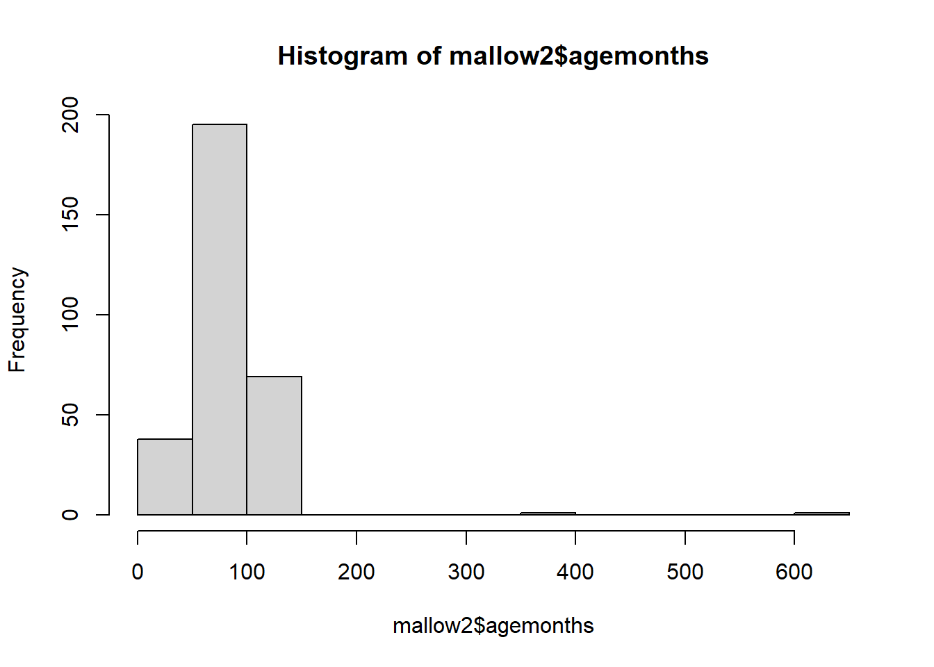
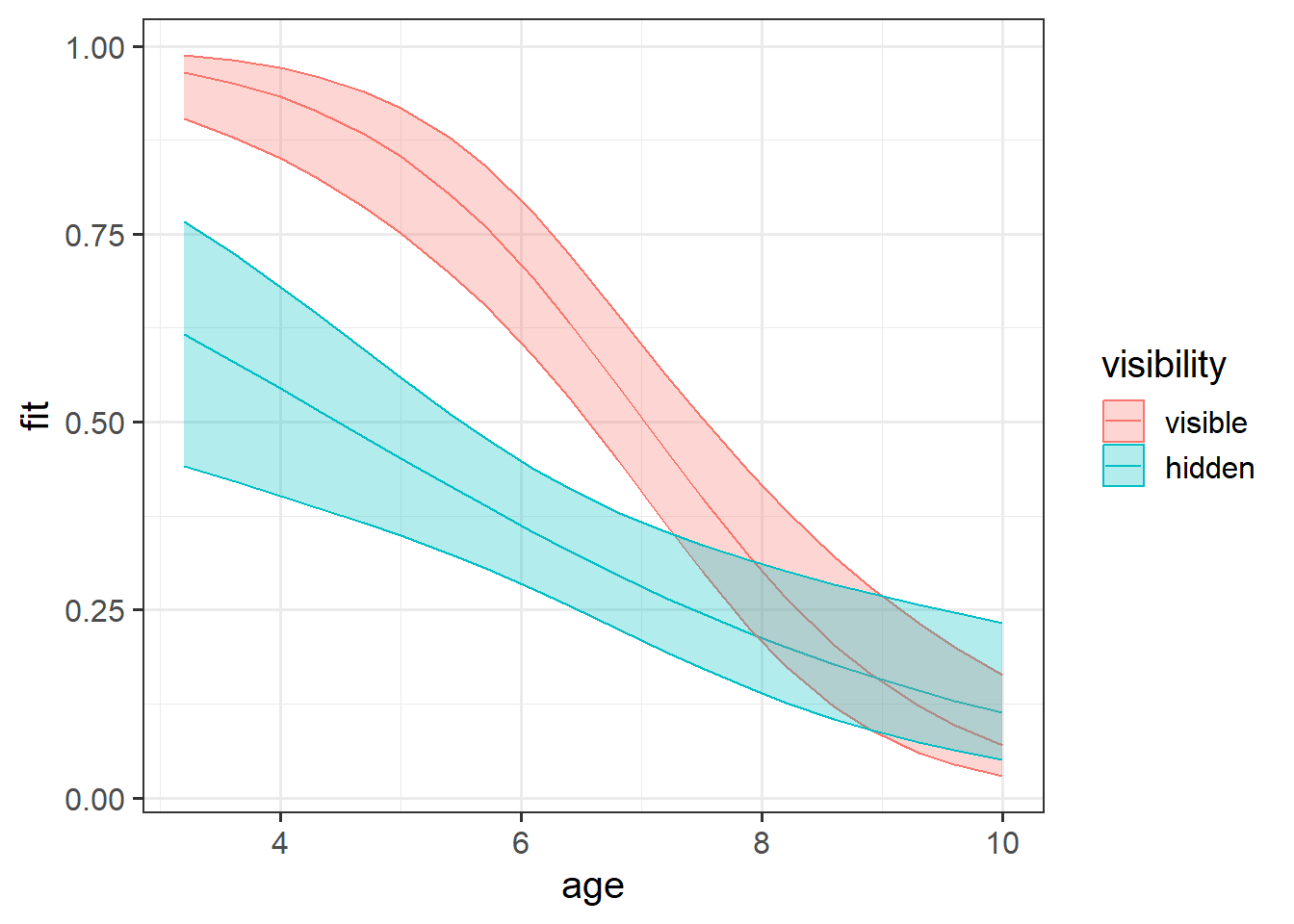
We already played with some marshmallow-related data in reading 10A. Here we are extending this study to investigate whether the visibility of the immediate reward moderates age effects on the ability to delay gratification (the ability to forgo an immediate reward for a greater reward at a later point).

304 children took part, ranging in ages from 3 to 10 years old. Each child was shown a marshmallow, and it was explained that they were about to be left alone for 10 minutes. They were told that they were welcome to eat the marshmallow while they were waiting, but if the marshmallow was still there after 10 minutes, they would be rewarded with two marshmallows.

For half of the children who took part, the marshmallow was visible for the entire 10 minutes (or until they ate it!). For the other half, the marshmallow was placed under a plastic cup.

The experiment took part at various times throughout the working day, and researchers were worried about children being more hungry at certain times of day, so they kept track of whether each child completed the task in the morning or the afternoon, so that they could control for this in their analyses.

The data are available at https://uoepsy.github.io/data/mallow2.csv.

Table 2:

Data dictionary for mallow2.csv

variable	description
name	Participant Name
agemonths	Age in months
timeofday	Time of day that the experiment took place ('am' = morning, 'pm' = afternoon)
visibility	Experimental condition - whether the marshmallow was 'visible' or 'hidden' for the 10 minutes
taken	Whether or not the participant took the marshmallow within the 10 minutes

Question 9

Read in the data, check, clean, plot, describe, explore.

Hints

• It’s good practice to set categorical variables as factors (see ).
  
• It might be easier to transform age into years rather than months (up to you!)

mallow2 <- read_csv("https://uoepsy.github.io/data/mallow2.csv")

We’ve only got one numeric variable here (age), so I’m going to plot that, and then tabulate the rest:

Something looks odd here.. a couple of very old children!

hist(mallow2$agemonths)

According to the design, our age range should be 3 to 10 years old. So here are all the participants over 10 years old (i.e. over 120 months old):

mallow2[mallow2$agemonths>120, ]

# A tibble: 2 × 5
  name   agemonths timeofday visibility taken 
  <chr>      <dbl> <chr>     <chr>      <chr> 
1 Martin       636 am        hidden     taken 
2 Josiah       396 pm        visible    waited

Aha… who knows how they got in there! We’ll deal with them in a minute..

The visibility variable looks as we would expect - half in each condition:

table(mallow2$visibility)

 hidden visible 
    152     152 

This looks off.. we have one mis-coded as “5 pm”, which I’m guessing should just be “pm”. And we have one at “noon”. There’s no way of knowing whether that was morning or afternoon, so I would be inclined to remove it.

table(mallow2$timeofday)

5 pm   am noon   pm 
   1  145    1  157 

And we can see that our outcome variable has got 2 unique values, which is what we expect.

table(mallow2$taken)

 taken waited 
   136    168 

So we need to:

1. replace “5 pm” with “pm” in timeofday
2. remove “noon” with NA in timeofday
3. remove Martin and Josiah.. they are not the population we’re interested in…
4. make any appropriate variables factors (good practice!)
5. while we’re there - I think I’ll also make an age variable that is in years rather than months

mallow2 <- 
  mallow2 |>
    mutate(
      age = agemonths/12,
      timeofday = factor(timeofday, 
                         levels=c("am","pm","5 pm"), # possible levels
                         labels = c("am","pm","pm")), # make the levels these
      visibility = factor(visibility, 
                          levels=c("visible","hidden")),
      taken = factor(taken, 
                     levels=c("waited","taken"))
    ) |>
  filter(agemonths <= 120, !is.na(timeofday))

KEEP TRACK
We’ve removed 3 observations entirely from the data. Two of these (Martin & Josiah) were clearly not representative of the population of interest. The other was one that had an unclear timeofday value. If we replaced it with NA, any analysis using that variable would not include that observation. And since we know we’re going to use timeofday in our analysis (and since it’s just 1 participant), it may be cleaner to just to start with a complete data.

When writing up, we would want to:

1. Detail any removal of observations and the reasons for doing so.
   
2. Describe the final dataset (if the final dataset contains NAs, then it’s also worth providing descriptions of the patterns of missingness).

mallow2 |>
  group_by(visibility) |>
  summarise(
    n = n(),
    mean_age = mean(age),
    sd_age = sd(age),
    percent_pm = sum(timeofday=="pm")/n()*100,
    percent_taken = sum(taken=="taken")/n()*100
  ) |>
  gt::gt() # this just a nice way to prettify tables 

visibility	n	mean_age	sd_age	percent_pm	percent_taken
visible	150	6.596667	1.820964	50.66667	56.00000
hidden	151	6.525938	1.922869	53.64238	33.11258

Question 10

Fit a model that you can use to address the research aims of the study.

Hints

Take a look back at the description of the study.

• What are we wanting to find out? How can we operationalise this into a model?
  • hint: ‘moderation’ is another word for ‘interaction’.
    
• Is there anything that we think it is important to account for?

mm1 <- glm(taken ~ timeofday + age * visibility, data = mallow2, family = binomial)

Question 11

What do you conclude?

Remember…

When you have an interaction Y ~ X1 + X2 + X3 + X2:X3 in your model, the coefficients that involved in the interaction (X2 and X3) represent the associations when the other variable in the interaction is zero.
The interaction coefficient itself represents the adjustment to these associations when we move up 1 in the other variable.

Here are the coefficients from the model we have fitted. We’ve exponentiated them so that they are in odds ratios.

exp(car::Confint(mm1))

                         Estimate        2.5 %       97.5 %
(Intercept)          560.14617820 83.620250311 4934.3779476
timeofdaypm            0.64074627  0.354154685    1.1383851
age                    0.41993953  0.312221939    0.5440124
visibilityhidden       0.01193413  0.001120213    0.1058236
age:visibilityhidden   1.64076760  1.189141035    2.3113652

From our coefficients, it looks like when the marshmallow is visible, the odds of taking the marshmallow are more than halved (0.42) for every year older a child is.

Compared to when the marshmallow is visible, the odds ratio associated with every additional year of age is 1.64 times bigger in the hidden-marshmallow condition.

This is a bit of a weird one to think about, but it means that instead of having an OR of 0.42 (as we do for the visible condition), for the hidden condition we have an OR that is \(0.42 \times 1.64 = 0.69\).

This is almost always going to be more easily presented as a plot of predicted probabilities:

Question 12

Write up the methods and results, providing a plot and regression table.

A template RMarkown file can be found at https://uoepsy.github.io/usmr/2324/misc/marshmallows.Rmd if you want it. It contains a list of questions try and make sure you answer in your write-up.

Optional Extras

Question 13

Below is the background and design to a study investigating how different types of more active learning strategies improve understanding, in comparison to just studying materials.

Fit an appropriate model to address the research aims, interpret it, make a plot, etc.

immersivelearning.csv

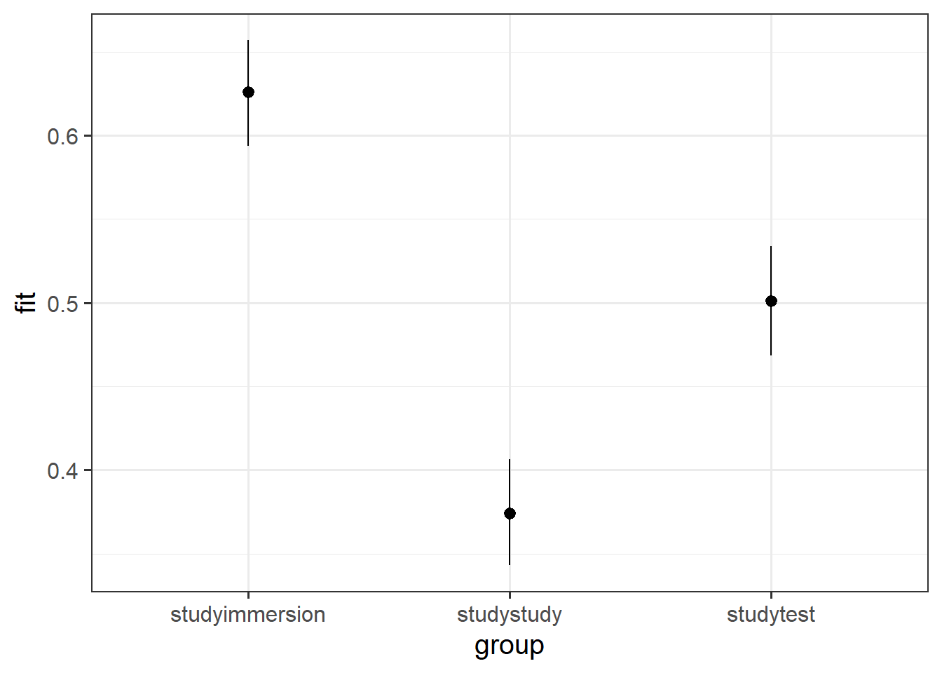
An experiment was run to investigate strategies for learning. Three groups of 30 participants were presented with materials on a novel language to learn.

All groups were given two hours of preparation time, after which their learning was assessed. The first group (studystudy) spent both hours studying the materials. The second group (studytest) spent the first hour studying the materials, and the second hour testing themselves on the materials. The third group (studyimmersion) spent the first hour studying the materials, and the second hour trying to converse with a native speaker of the language (they were not permitted to attempt to converse in any other language during this time).

After the two hours were up, participants were the assessed via a series of 30 communication tasks. The number of tasks each participant got correct was recorded.

Information on two potential covariates was also included - previous language learning experience (novice/experienced), and cognitive aptitude (a 20 item questionnaire leading to a standardised test score).

The data are available at https://uoepsy.github.io/data/immersivelearning.csv.

Table 3:

Data dictionary: immersivelearning.csv

variable	description
PID	Participant ID number
group	Experimental group (studystudy = 2 hours of study, studytest = 1 hour study, 1 hour testing, studyimmersion = 1 hour study, 1 hour conversing)
plle	Previous language learning experience (novice or experienced)
cog_apt	Cognitive Aptitude (Standardised Z Score)
n_correct	Number of the 30 communication tasks that each participant correctly completed

Hints

• This might not be binary (0 or 1), but it’s binomial (“how many success in 30 trials”).
  
• See the optional box under logistic regression in 10A #fitting-glm-in-r for how to fit a binomial model to data like this.

Below is the code we would use to investigate this. Some of these decisions you might make differently, and that is okay - the important thing is to clearly explain and justify the decision we make.

immers <- read_csv("https://uoepsy.github.io/data/immersivelearning.csv")

immers <- immers |> mutate(
  fct_relevel(factor(group), "studystudy")
)

mst1 = glm(cbind(n_correct,30-n_correct) ~ plle+cog_apt+group,
    data = immers, family=binomial)

summary(mst1)

Call:
glm(formula = cbind(n_correct, 30 - n_correct) ~ plle + cog_apt + 
    group, family = binomial, data = immers)

Coefficients:
                Estimate Std. Error z value Pr(>|z|)    
(Intercept)      0.60154    0.10591   5.680 1.35e-08 ***
pllenovice      -0.10897    0.09905  -1.100    0.271    
cog_apt         -0.03194    0.03725  -0.857    0.391    
groupstudystudy -1.02919    0.09798 -10.504  < 2e-16 ***
groupstudytest  -0.51064    0.09661  -5.286 1.25e-07 ***
---
Signif. codes:  0 '***' 0.001 '**' 0.01 '*' 0.05 '.' 0.1 ' ' 1

(Dispersion parameter for binomial family taken to be 1)

    Null deviance: 644.49  on 89  degrees of freedom
Residual deviance: 529.99  on 85  degrees of freedom
AIC: 862.24

Number of Fisher Scoring iterations: 4

effect(term = "group", mod = mst1) |>
  as.data.frame() |>
  ggplot(aes(x=group, y=fit,ymin=lower,ymax=upper))+
  geom_pointrange()

Question 14

People and behaviours are a lot more difficult to predict than something like, say, the colour of different wines.

Build a model that predicts the colour of wine based on all available information. How accurately can it predict wine colours?

(Generally speaking, this question doesn’t reflect how we do research in psychology. Ideally, we would have a theoretical question that motivates the inclusion (and testing of) specific predictors.)

usmr_wines.csv

You can download a dataset of 6497 different wines (1599 red, 4898 white) from https://uoepsy.github.io/data/usmr_wines.csv.

It contains information on various physiochemical properties such as pH, a measure of level of sulphates, residual sugar, citric acid, volatile acidity and alcohol content, and also quality ratings from a sommelier (wine expert). All the wines are vinho verde from Portugal, and the data was collected between 2004 and 2007.

Hints

• glm(outcome ~ ., data = mydata) is a shorthand way of putting all variables in the data in as predictors.
  
• See the lecture slides for an example of how we can get a number for “how accurately can my model predict”.

Below is the code we would use to investigate this. Some of these decisions you might make differently, and that is okay - the important thing is to clearly explain and justify the decision we make.

wines <- read_csv("https://uoepsy.github.io/data/usmr_wines.csv")

wines <- 
  wines |> 
  mutate(
    col = factor(col, levels=c("white","red"))
  )

winemod <- glm(col ~ ., data = wines, family = binomial)

# in logit units
guess <- predict(winemod)
# logit 0 is p of .5:
guess <- ifelse(guess > 0, "red", "white")
# how many predicted colours match the observed colours??
hits <- sum(guess == wines$col)
# what percentage?  
hits/length(wines$col)

[1] 0.936894

Footnotes

1. the colon here means “look in the car package and use the Confint() function. It saves having to load the package with library(car)