Exercises: Interactions!

Processing a hangover

Dataset: hangover_speed.csv

How is hours of sleep associated with processing speed? Is this dependent upon whether or not alcohol was consumed the previous night? 107 participants completed the Symbol Digit Modalities Task (SDMT), a measure of processing speed. Participants also recorded how many hours they had slept the previous night (to the nearest 15 mins), and whether or not they had consumed alcohol.

The dataset is available at https://uoepsy.github.io/data/hangover_speed.csv.

variable	description
hrs_sleep	hours slept the previous night (to the nearest 15 mins)
alc	was alcohol consumed the previous evening? ('y'=yes, 'n'=no)
sdmt	score on the Symbol Digit Modalities Task (SDMT), a measure of processing speed (range 0 to 100)

Question 1

Read in the data and provide some simple descriptives.

Hints

• What is the mean score on the SDMT, what is the variability in scores?
  
• How many people had alcohol the previous night?
  
• How many hours did people sleep on average? Did this vary between the drinkers and the non-drinkers?

Here’s our data. Everything looks within plausible ranges for our two continuous variables hrs_sleep and sdmt.

hodat <- read_csv("https://uoepsy.github.io/data/hangover_speed.csv")

We can get the means and SDs for hours slept and the SDMT:

library(psych)
describe(hodat |> select(-alc))

          vars   n  mean    sd median trimmed   mad   min  max range skew
hrs_sleep    1 107  7.20  1.20   7.25    7.18  1.11  4.25 10.5  6.25 0.20
sdmt         2 107 54.59 12.13  53.00   54.23 10.38 22.00 86.0 64.00 0.28
          kurtosis   se
hrs_sleep     0.07 0.12
sdmt          0.08 1.17

We can see that 57% of participants didn’t drink, and 43% of them did:

table(hodat$alc)

 n  y 
61 46 

And it doesn’t look like they differed very much in their sleep times:

hodat |> group_by(alc) |>
  summarise(
    slept = mean(hrs_sleep)
  )

# A tibble: 2 × 2
  alc   slept
  <chr> <dbl>
1 n      7.12
2 y      7.30

Question 2

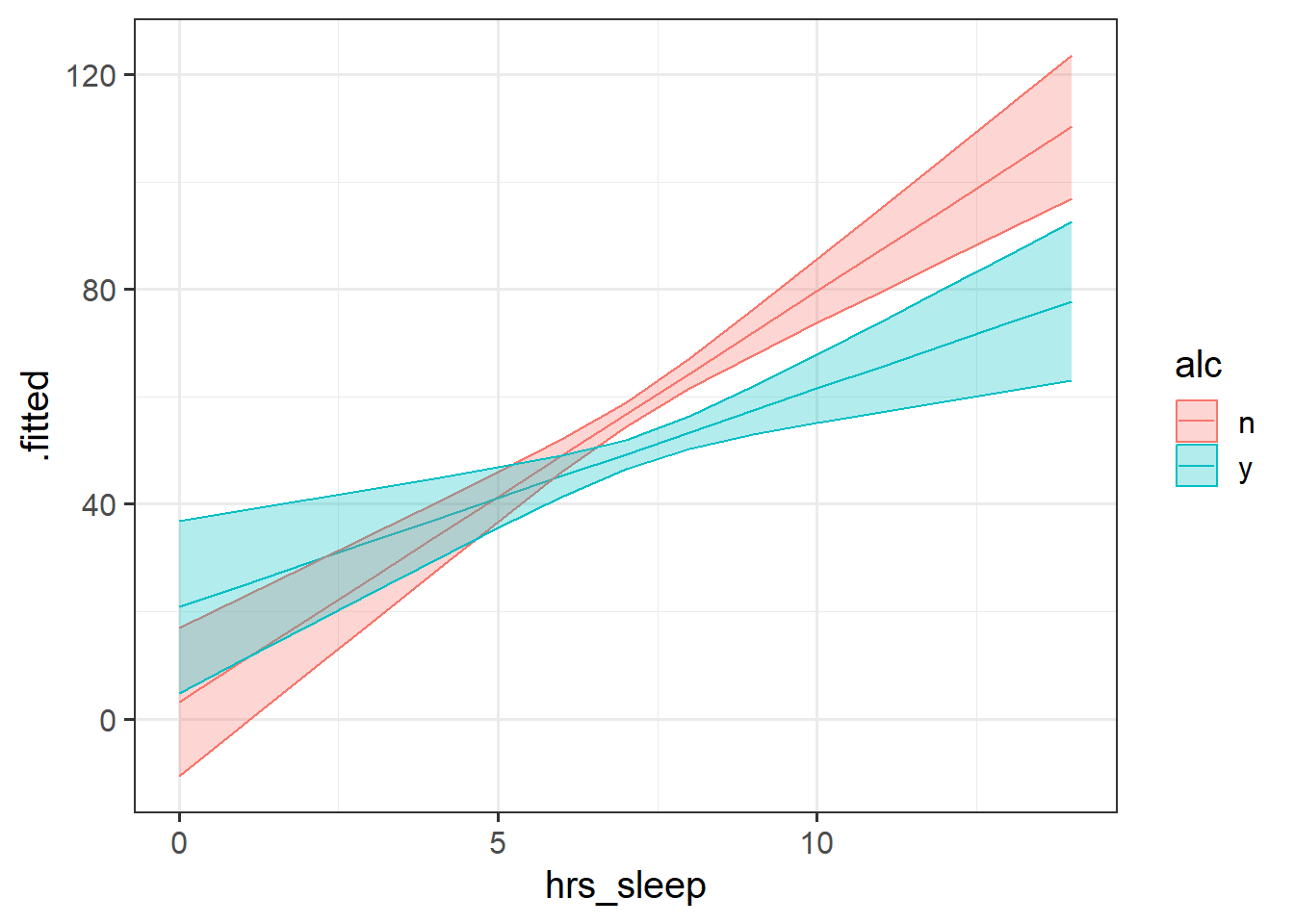
Make a plot of SDMT predicted by hours slept, and colour the points by whether or not the participants had drank alcohol.

Can you plot a separate lm line on the graph using geom_smooth for each group (alcohol v no alcohol)?

Hints

• to make geom_smooth() fit a linear model (lm), remember to use geom_smooth(method=lm).
  
• if you have the grouping in the aes(), then when you add geom_smooth() it should make a different one for each group!

ggplot(hodat, aes(x = hrs_sleep, y = sdmt, col = alc)) +
  geom_point() +
  geom_smooth(method=lm)

Question 3

Adding a different geom_smooth(method=lm) for each group is just fitting a different model to each groups’ data - i.e. a slope of sdmt~hrs_sleep for the drinkers and a slope for the non-drinkers.

But we actually want to test if the two slopes are different, and for that we need to create a model which includes the appropriate interaction term.
Fit the model to examine whether the association between hrs_sleep and sdmt is different depending upon alcohol consumption.

Hints

This is the same logic as the air-pollution & APOE-4 example in 9A #it-depends.

mod_int <- lm(sdmt ~ hrs_sleep * alc, data = hodat)
summary(mod_int)

Call:
lm(formula = sdmt ~ hrs_sleep * alc, data = hodat)

Residuals:
     Min       1Q   Median       3Q      Max 
-23.3384  -5.2919  -0.2911   6.6458  19.7389 

Coefficients:
               Estimate Std. Error t value Pr(>|t|)    
(Intercept)      3.1496     6.9631   0.452   0.6520    
hrs_sleep        7.6499     0.9643   7.933 2.71e-12 ***
alcy            17.7151    10.6874   1.658   0.1004    
hrs_sleep:alcy  -3.5867     1.4593  -2.458   0.0156 *  
---
Signif. codes:  0 '***' 0.001 '**' 0.01 '*' 0.05 '.' 0.1 ' ' 1

Residual standard error: 8.914 on 103 degrees of freedom
Multiple R-squared:  0.4753,    Adjusted R-squared:   0.46 
F-statistic:  31.1 on 3 and 103 DF,  p-value: 2.136e-14

Question 4

Interpret each coefficient from your model.

Hints

Our interaction involves a continuous variable (hrs_sleep) and a binary variable (alc). An interpretation of a similar example is in 9A #interpretation.

summary(mod_int)

Coefficients:
               Estimate Std. Error t value Pr(>|t|)    
(Intercept)      3.1496     6.9631   0.452   0.6520    
hrs_sleep        7.6499     0.9643   7.933 2.71e-12 ***
alcy            17.7151    10.6874   1.658   0.1004    
hrs_sleep:alcy  -3.5867     1.4593  -2.458   0.0156 *  
---

coefficient	estimate	interpretation
(Intercept)	3.15	A non-drinker who slept 0 hours is estimated to have an SDMT score of 3.1 - note this is not significantly different from zero
hrs_sleep	7.65	For every additional hour slept, non-drinkers scores on SDMT are estimated to increase by 7.6
alcy	17.72	drinkers who slept zero hours are estimated to have 17.7 higher scores on SDMT than non-drinkers who slept zero hours - note this is not significantly different from zero
hrs_sleep:alcy	-3.59	For every additional hour's sleep, drinkers scores on SDMT increase by 3.6 *less* than they do for non-drinkers

Question 5

Construct a plot of the model estimated associations between hours-slept and SDMT for drinkers and non-drinkers.

Because we have nothing else in our model, this should end up looking exactly the same as our initial plot in Question 2!

Hints

It all follows the same logic as we have used before:

1. make a dataframe of the values of the predictors that we wish to plot across
2. using augment(), add to that the predicted values of the model, and the associated confidence intervals
3. shove it all in ggplot!

Because we are wanting to plot across multiple predictors (i.e. we want to plot across a range of hrs_slept and both values of alc), try using expand_grid().

Play around with this to see what it does:

# A tibble: 15 × 2
   continuous binary
        <int> <chr> 
 1          1 dog   
 2          1 cat   
 3          1 parrot
 4          2 dog   
 5          2 cat   
 6          2 parrot
 7          3 dog   
 8          3 cat   
 9          3 parrot
10          4 dog   
11          4 cat   
12          4 parrot
13          5 dog   
14          5 cat   
15          5 parrot

If you get stuck, a very similar example is in 9A #visualisation.

# plot data
plotdat <- expand_grid(
  hrs_sleep = 0:14,
  alc = c("n","y")
)
# plot
broom::augment(mod_int, newdata = plotdat, interval="confidence") |>
  ggplot(aes(x= hrs_sleep, y = .fitted, 
             col = alc, fill = alc)) + 
  geom_line() +
  geom_ribbon(aes(ymin=.lower,ymax=.upper), alpha=.3)

Question 6

No one in our dataset has slept zero hours, and i’m probably not interested in differences between drinkers/non-drinkers who never sleep.

Refit the model to adjust the intercept to a more meaningful value. Everyone always goes on about 8 hours of sleep being the minimum?

How has the interpretation of your coefficient(s) changed?

Hints

See 9A #mean-centering for an example of mean-centering a predictor in the interaction. Remember that there are multiple ways to do this - you could make a new variable first, or you could do it all inside the model.

If we want to recenter our hrs_sleep variable on 8 hours, we could either create a new variable which is hrs_sleep - 8 (which would therefore make everyone who slept 8 hours be given a value of 0 in the variable), or we could do it in the model:

re-centering first

hodat <- 
  hodat |>
    mutate(
      hrs_8 = hrs_sleep - 8
    )

mod_int2 <- lm(sdmt ~ hrs_8 * alc, data = hodat)

doing it all in the model

mod_int2 <- lm(sdmt ~ I(hrs_sleep-8) * alc, data = hodat)

summary(mod_int2)

Coefficients:
                      Estimate Std. Error t value Pr(>|t|)    
(Intercept)            64.3487     1.4206  45.297  < 2e-16 ***
I(hrs_sleep - 8)        7.6499     0.9643   7.933 2.71e-12 ***
alcy                  -10.9786     2.0800  -5.278 7.27e-07 ***
I(hrs_sleep - 8):alcy  -3.5867     1.4593  -2.458   0.0156 *  
---

coefficient	estimate	interpretation
(Intercept)	64.35	A non-drinker who slept 8 hours is estimated to have an SDMT score of 64.3
I(hrs_sleep - 8)	7.65	For every additional hour slept, non-drinkers scores on SDMT are estimated to increase by 7.6
alcy	-10.98	drinkers who slept 8 hours are estimated to have 11 lower scores on SDMT than non-drinkers who slept 8 hours
I(hrs_sleep - 8):alcy	-3.59	For every additional hour's sleep, drinkers scores on SDMT increase by 3.6 *less* than they do for non-drinkers

The monkeys are back!

Data: ctmtoys.csv

So far, we have analysed the data for two studies (not real!) of the inquisitive nature of monkeys. Initially (week 5 exercises), Liu, Hajnosz & Li (2023) investigated age differences in exploration of novel objects, and found that older monkeys spend on average less time playing with a novel object than their younger counterparts (we looked at this with both with the linear effect of age in years, and by comparing adults to juveniles). Following this Liu, Hajnosz, Xu & Li (2023) wanted to see if monkeys showed a preference for different types of object (i.e. ones with moving parts vs ones that are soft). They found that, after accounting for differences due to age, monkeys showed a significant preference for toys with moving parts in comparison to soft toys.

Xu, Li, Liu & Hajnosz (2023c) are again asking for our help, and this time with a bigger study, of 216 monkeys. They are interested in whether the preference for mechanical toys over soft toys is different for different species of monkey. Both the previous studies were conducted on Rhesus Macaques (a species that have adapted very well to human dominated landscapes), so this study has re-run the same experiment on 69 Capuchin monkeys, 71 Tamarin monkeys and 76 Macaques.

The aim of this study is to investigate the following question:

Are preferences between soft toys vs mechanical toys different for different species of monkey?

The data is available at https://uoepsy.github.io/data/ctmtoys.csv and contains the variables described in Table 1

Table 1:

Data dictionary for ctmtoys.csv

variable	description
name	Monkey Name
age	Age of monkey in years
species	Species (capuchin, macaque, tamarin)
obj_type	Type of novel object given (mechanical / soft)
obj_colour	Main colour of object (red / green / blue)
obj_size	Size of object in cm (length of largest dimension of the object)
exptime	Time (in minutes) spent exploring the object

Question 7

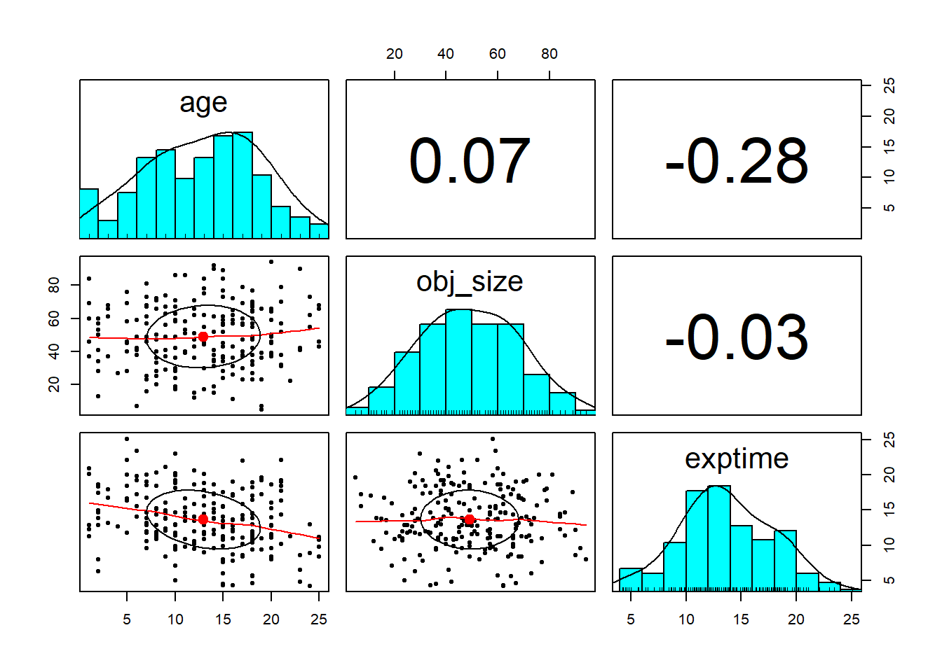
As always, begin by reading in your data and making some exploratory plots to get an idea of the distributions we’re dealing with.

Everything looks okay in terms of our variable ranges here:

ctmtoys <- read_csv("https://uoepsy.github.io/data/ctmtoys.csv")
summary(ctmtoys)

     name                age          species            obj_type        
 Length:216         Min.   : 1.00   Length:216         Length:216        
 Class :character   1st Qu.: 8.00   Class :character   Class :character  
 Mode  :character   Median :13.00   Mode  :character   Mode  :character  
                    Mean   :12.92                                        
                    3rd Qu.:18.00                                        
                    Max.   :25.00                                        
  obj_colour           obj_size        exptime     
 Length:216         Min.   : 5.00   Min.   : 4.20  
 Class :character   1st Qu.:36.00   1st Qu.:11.00  
 Mode  :character   Median :49.00   Median :13.45  
                    Mean   :49.06   Mean   :13.66  
                    3rd Qu.:62.25   3rd Qu.:16.75  
                    Max.   :94.00   Max.   :25.10  

Let’s shove it in pairs.panels:

ctmtoys |> 
  select(age, obj_size, exptime) |>
  psych::pairs.panels()

And let’s tabulate obj_type and species:

ctmtoys |>
  select(obj_type, species) |>
  table()

            species
obj_type     capuchin macaque tamarin
  mechanical       33      43      32
  soft             36      33      39

Question 8

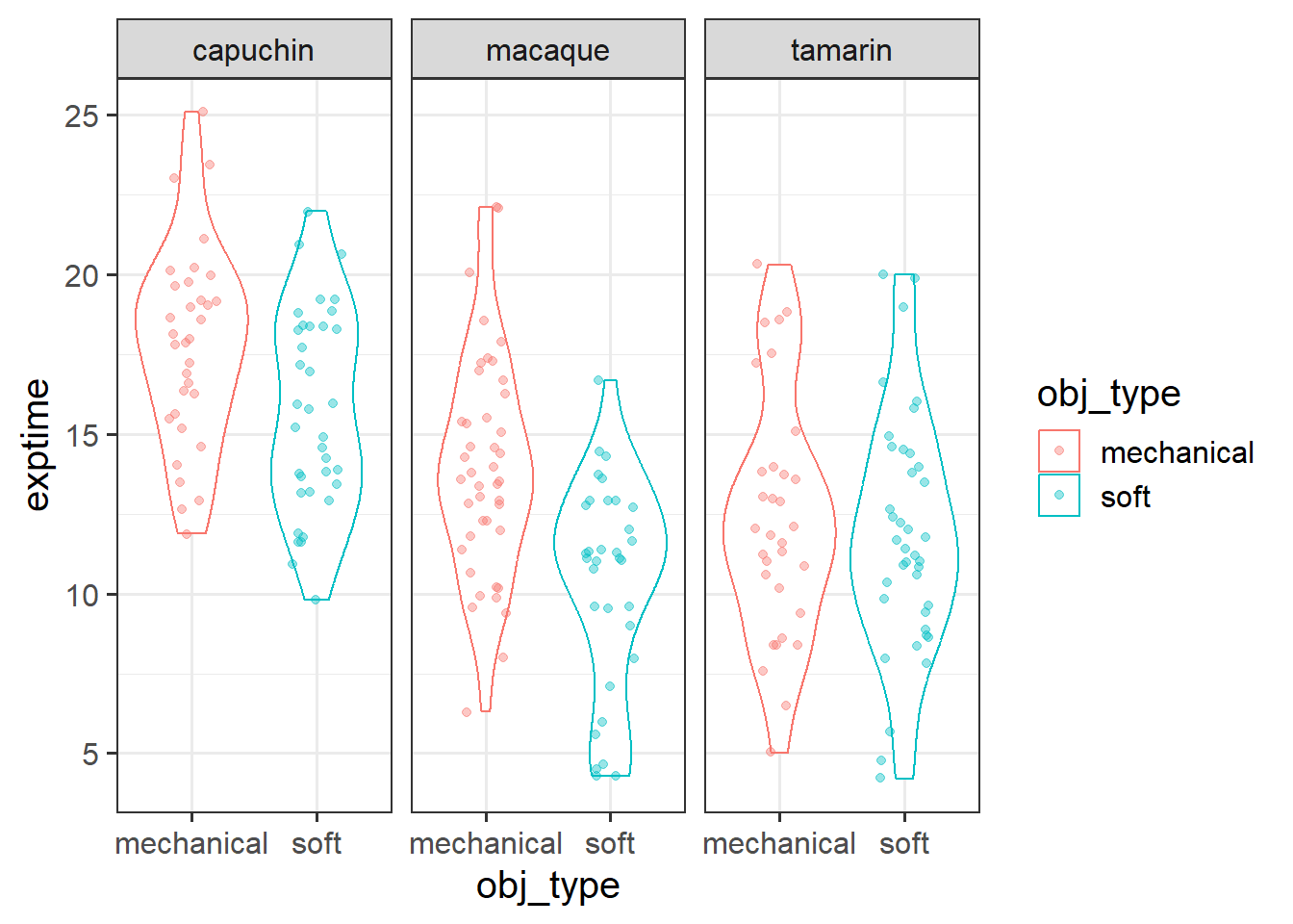
Try making some initial exploratory plots of the relationships in the data that are relevant to the research question.

Hints

We’re wanting to plot exploration_time and obj_type here, but we’re also wanting to show it for each species. This means we’ll need things like colours, facets, etc.

From initial exploration - it looks like capuchins are generally spending more time playing with the objects (of both types).
The slight preference for mechanical toys seems to be present Capuchins and Macaques, but it’s less clear in the Tamarins.

ggplot(ctmtoys, aes(x = obj_type, y = exptime, 
                    col = obj_type)) +
  geom_violin() + 
  geom_jitter(width=.2, alpha=.4) + 
  facet_wrap(~species)

All of this is just initial speculation, however - we haven’t considered lots of things such as the distributions of ages between the species, or whether they all saw objects of similar sizes and colours. These things could make these plots appear to show relationships that are actually driven by other things. They could also make these plots hide relationships that are present once these things are controlled for.

Question 9

Fit an appropriate model to address the research question.
Think about what we already know from previous studies - we’ll likely want to control for age and for other aspects of objects like size and colour.

Then think about the specific research question and what is needed to test it.

modelmonkey <- lm(exptime ~ age + obj_size + obj_colour +
                obj_type * species, data = ctmtoys)

Question 10

Do species differ in their preference for different types of object?

Hints

Think about how the question is worded - there’s no “how”/“what” etc, it’s just “are there differences?” (this is just the same as we did last week, and in 8B #testing-group-differences - try a model comparison?).

Let’s compare a reduced model without the interaction to our model with the interaction:

modelmonkey0 <- lm(exptime ~ age + obj_size + obj_colour +
                obj_type + species, data = ctmtoys)

anova(modelmonkey0, modelmonkey)

Analysis of Variance Table

Model 1: exptime ~ age + obj_size + obj_colour + obj_type + species
Model 2: exptime ~ age + obj_size + obj_colour + obj_type * species
  Res.Df    RSS Df Sum of Sq      F  Pr(>F)  
1    208 2339.2                              
2    206 2257.0  2    82.136 3.7483 0.02518 *
---
Signif. codes:  0 '***' 0.001 '**' 0.01 '*' 0.05 '.' 0.1 ' ' 1

Species significantly differed in the extent to which exploration time varied between different types of object (\(F(2, 206)=3.75, p=0.0252\)).

Question 11

Now, we want to know how species differ in their preferences for different types of object?

Take a look at the model coefficients.

summary(modelmonkey)

Call:
lm(formula = exptime ~ age + obj_size + obj_colour + obj_type * 
    species, data = ctmtoys)

Residuals:
   Min     1Q Median     3Q    Max 
-8.959 -2.348 -0.045  2.015  9.745 

Coefficients:
                            Estimate Std. Error t value Pr(>|t|)    
(Intercept)                 19.33098    1.03529  18.672  < 2e-16 ***
age                         -0.16464    0.03961  -4.157 4.73e-05 ***
obj_size                     0.01122    0.01252   0.896   0.3712    
obj_colourgreen             -0.14963    0.55815  -0.268   0.7889    
obj_colourred               -0.19467    0.55887  -0.348   0.7279    
obj_typesoft                -1.96193    0.80839  -2.427   0.0161 *  
speciesmacaque              -3.90720    0.77012  -5.073 8.70e-07 ***
speciestamarin              -5.08712    0.82839  -6.141 4.16e-09 ***
obj_typesoft:speciesmacaque -1.51124    1.11855  -1.351   0.1782    
obj_typesoft:speciestamarin  1.53986    1.15128   1.338   0.1825    
---
Signif. codes:  0 '***' 0.001 '**' 0.01 '*' 0.05 '.' 0.1 ' ' 1

Residual standard error: 3.31 on 206 degrees of freedom
Multiple R-squared:  0.392, Adjusted R-squared:  0.3655 
F-statistic: 14.76 on 9 and 206 DF,  p-value: < 2.2e-16

In our model coefficients, both interaction terms are non-significant.
But we just said before that in the previous question that there is an interaction (we got our F test for it).

The coefficients above are telling us that, compared to the reference species (capuchins), neither macaques nor tamarins show significant differences in their preference for mechanical toys vs soft toys.

But while macaques and tamarins may not be different from capuchins, it is entirely possible that macaques and tamarins could be different from each other?

Question 12

Model coefficients are always relative to some reference point (i.e. capuchins with mechanical toys).

1. Change the reference point to Macaques with soft toys.
   
2. Refit the model.
3. Interpret the coefficients.

We always get to choose which level we want as a reference. Sometimes, this will be easy because on level represents the norm/status quo. In this context, Macaques is possibly a more useful reference, given that the study description earlier mentioned the previous studies were conducted on Macaques.

Re-levelling obj_type to have “soft” as the reference won’t make much difference - it will just swap the signs of the coefficients (comparing mechanical to soft, as opposed to comparing soft to mechanical).

ctmtoys <- 
  ctmtoys |>
  mutate(
    species = fct_relevel(species, "macaque"),
    obj_type = fct_relevel(obj_type, "soft")
  )

lm(exptime ~ age + obj_size + obj_colour +
                obj_type * species, data = ctmtoys) |>
  summary()

Call:
lm(formula = exptime ~ age + obj_size + obj_colour + obj_type * 
    species, data = ctmtoys)

Residuals:
   Min     1Q Median     3Q    Max 
-8.959 -2.348 -0.045  2.015  9.745 

Coefficients:
                                   Estimate Std. Error t value Pr(>|t|)    
(Intercept)                        11.95061    1.01699  11.751  < 2e-16 ***
age                                -0.16464    0.03961  -4.157 4.73e-05 ***
obj_size                            0.01122    0.01252   0.896  0.37122    
obj_colourgreen                    -0.14963    0.55815  -0.268  0.78890    
obj_colourred                      -0.19467    0.55887  -0.348  0.72794    
obj_typemechanical                  3.47317    0.76957   4.513 1.07e-05 ***
speciescapuchin                     5.41843    0.80728   6.712 1.83e-10 ***
speciestamarin                      1.87117    0.80555   2.323  0.02116 *  
obj_typemechanical:speciescapuchin -1.51124    1.11855  -1.351  0.17816    
obj_typemechanical:speciestamarin  -3.05110    1.11480  -2.737  0.00674 ** 
---
Signif. codes:  0 '***' 0.001 '**' 0.01 '*' 0.05 '.' 0.1 ' ' 1

Residual standard error: 3.31 on 206 degrees of freedom
Multiple R-squared:  0.392, Adjusted R-squared:  0.3655 
F-statistic: 14.76 on 9 and 206 DF,  p-value: < 2.2e-16

These coefficients show us that Macaques tend to spend 3.5 more minutes playing with mechanical toys than soft toys, and that Capuchins do not significantly differ in this respect, but Tamarins do. Relative to Macaques, Tamarins spend 3.05 less additional time with mechanical toys compared to soft toys.

Question 13

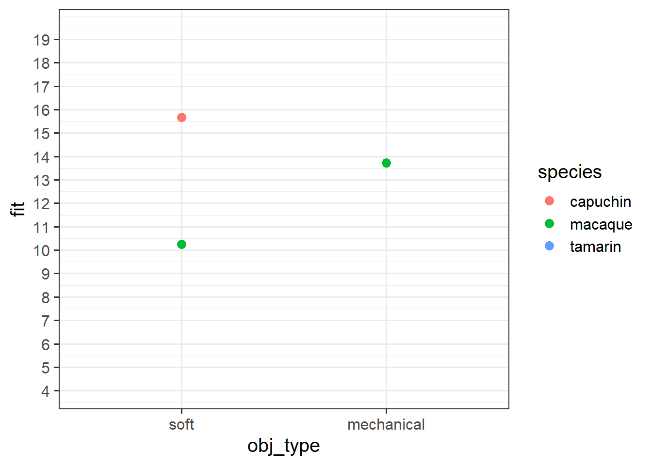
The interpretation of interaction coefficients tends to be quite confusing, and invariably it helps to tie these to a visualisation. We’re going to do it manually here, because it’s a very useful learning exercise.

Below are our coefficients of interest from the model, when the reference level for obj_type is “soft” and for species is “macaque”.

...
obj_typemechanical                  3.47317    0.76957   4.513 1.07e-05 ***
speciescapuchin                     5.41843    0.80728   6.712 1.83e-10 ***
speciestamarin                      1.87117    0.80555   2.323  0.02116 *  
obj_typemechanical:speciescapuchin -1.51124    1.11855  -1.351  0.17816    
obj_typemechanical:speciestamarin  -3.05110    1.11480  -2.737  0.00674 ** 

Grab a piece of paper, and draw the points for each species & obj_type combination, relative to the reference point.
Start with the plot below:

The coefficient “obj_typemechanical” tells us the difference between soft and mechanical toys when species is zero - i.e., when it is at the reference level (macaques).

So we know that macaques spend 3.5 more minutes with mechanical toys compared to soft toys:

The coefficient “speciescapuchin” tells us the difference between capuchins and macaques, when obj_type is zero - i.e., when it is at the reference level (soft).

So we know that capuchins spend 5.4 more minutes with soft toys compared to macaques with soft toys:

The coefficient “speciestamarin” tells us the difference between tamarins and macaques, when obj_type is zero - i.e., when it is at the reference level (soft).

So we know that tamarins spend 1.9 more minutes with soft toys compared to macaques with soft toys:

The coefficient “obj_typemechanical:speciescapuchin” tells us the difference between capuchins and macaques’ soft-vs-mechanical differences.
i.e. when moving from macaques to capuchins, the soft-to-mechanical difference changes by this much.

So we know that whereas macaques spend 3.5 more minutes with mechanical toys compared to soft toys, for capuchins this is 1.5 minutes less.
So rather than going up 3.5, we go up \(3.5-1.5=2\).

However, this is non-significant. So the difference could easily just be 0 - i.e. they could increase by the same 3.5 minutes as Macaques do. So we know that the uncertainty here should also capture as if Capuchins and Macaques have the same increases from soft to mechanical.

The coefficient “obj_typemechanical:speciestamarin” tells us the difference between tamarins and macaques’ soft-vs-mechanical differences.
i.e. when moving from macaques to tamarins, the soft-to-mechanical difference changes by this much.

So we know that whereas macaques spend 3.5 more minutes with mechanical toys compared to soft toys, for tamarins this is 3.05 minutes less.
So rather than going up 3.5, we go up \(3.5-3.05=0.45\):

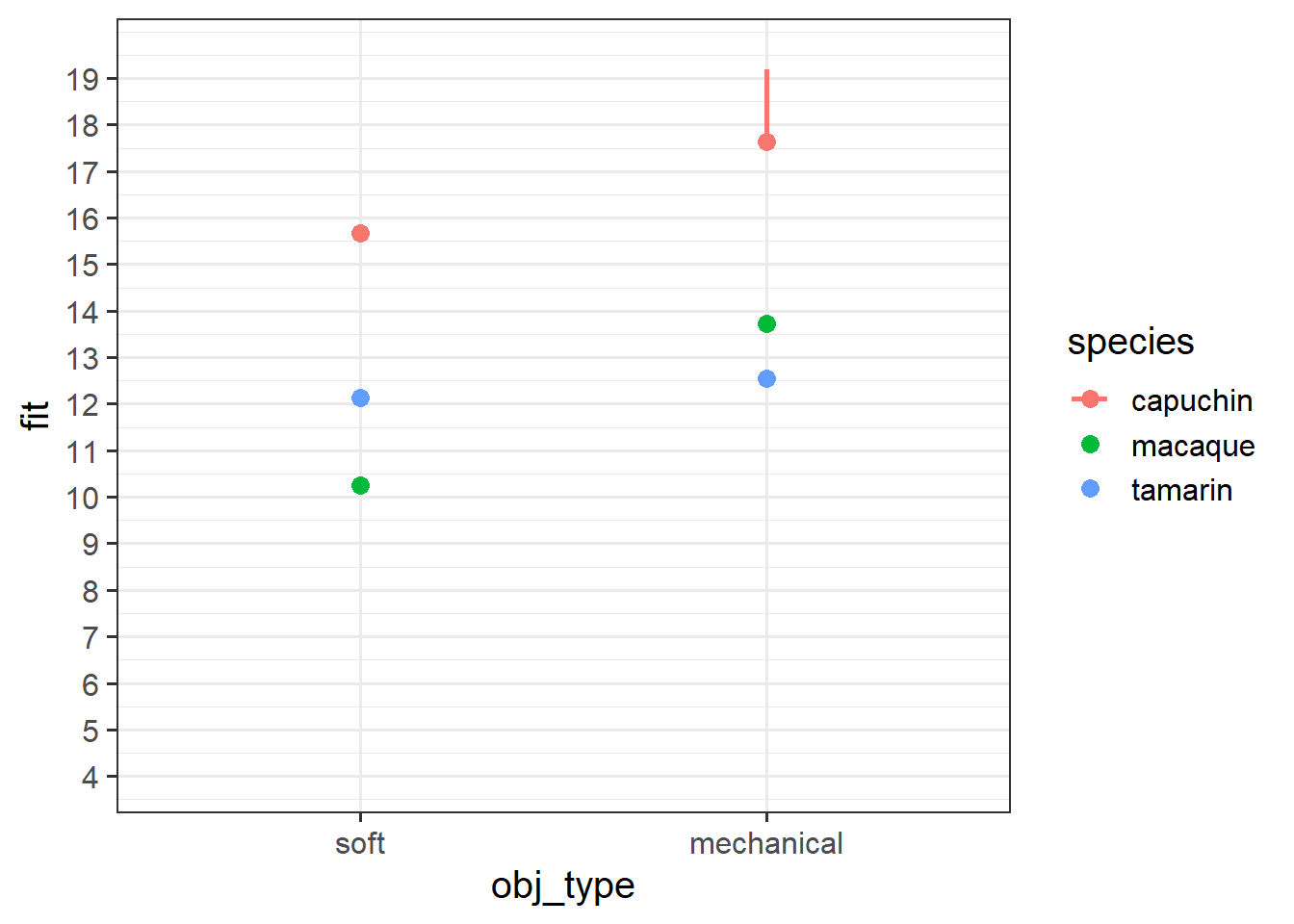
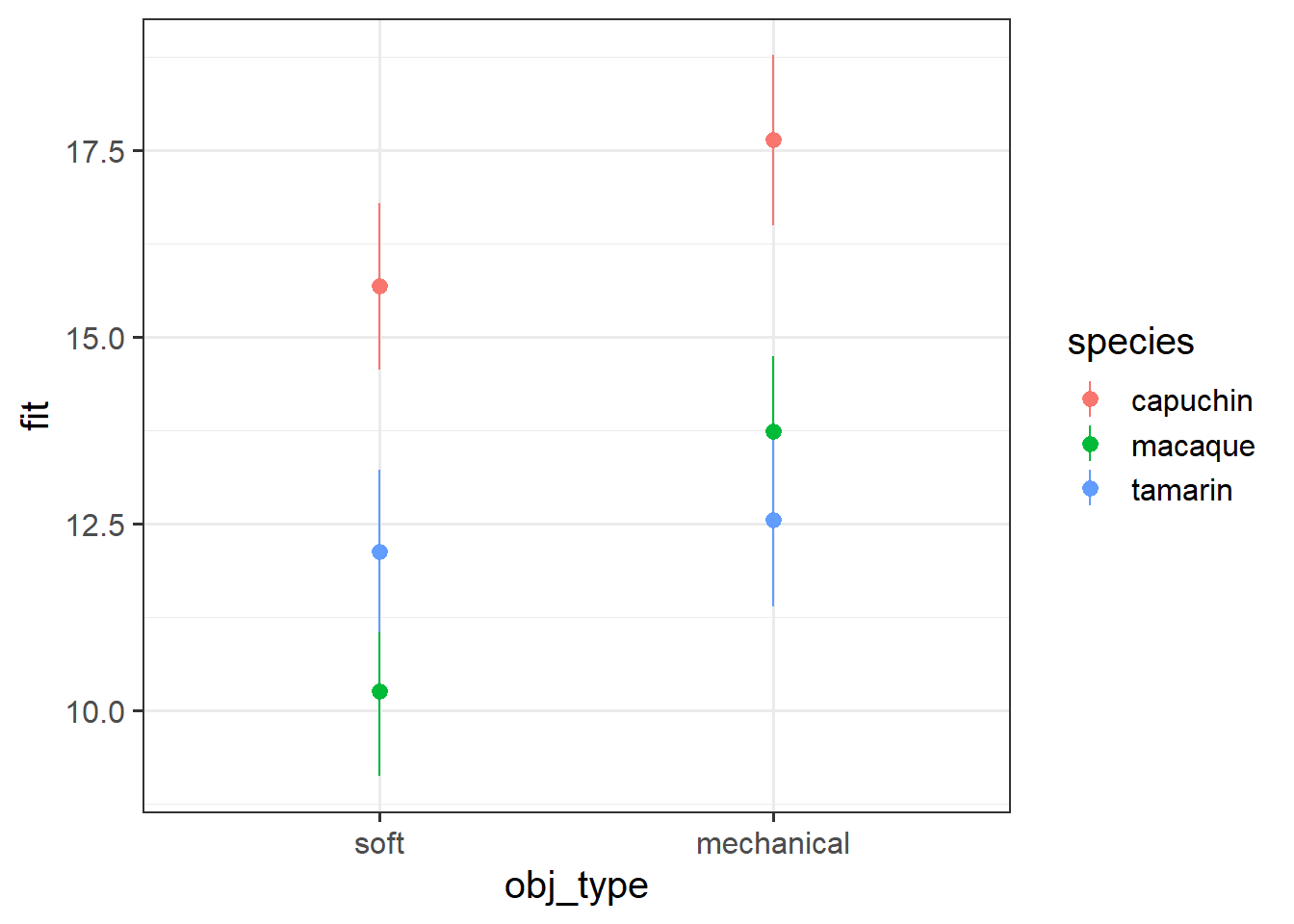
Question 14

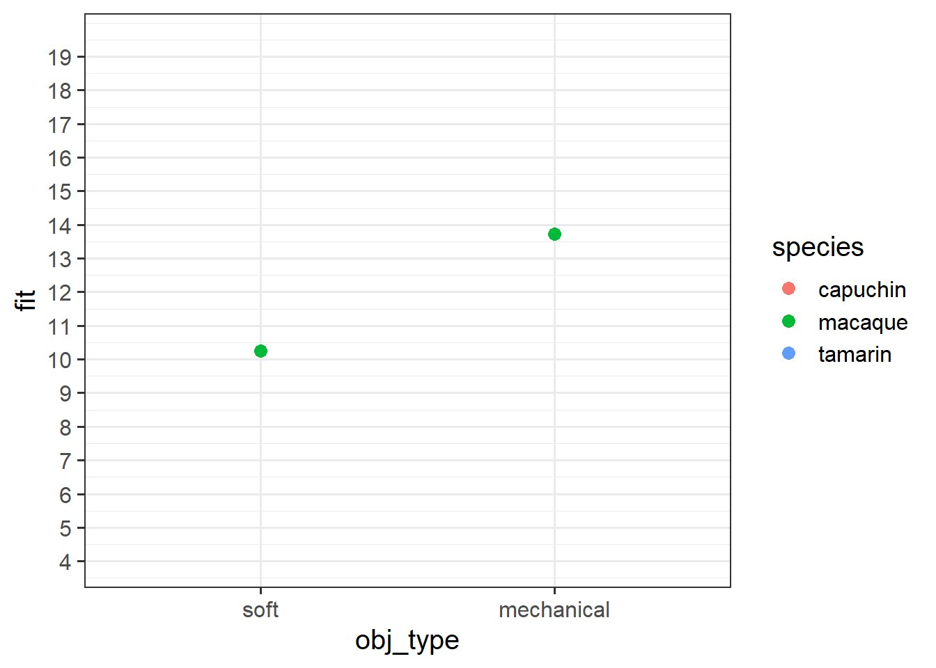
Okay, now let’s make a plot in R.

Try running this code in pieces to see what each bit does, and then running it all at once to get the plot.

Does it match with what you sketched in the previous question?

library(effects)
effect("obj_type*species",modelmonkey) |>
  as.data.frame() |>
  mutate(
    obj_type = fct_relevel(factor(obj_type), "soft")
  ) |>
  ggplot(aes(x=obj_type, y=fit, col=species)) +
  geom_pointrange(aes(ymin=lower,ymax=upper))

Why use the effects package?

Up to now, when we’ve been plotting our associations of interest we’ve been choosing to construct our plots at the mean of our other predictors.

However, in our current monkey model, we’ve also got a categorical covariate (obj_colour) in our model. What should we do with that?

plotdat <- expand_grid(
  age = mean(ctmtoys$age),
  obj_size = mean(ctmtoys$obj_size),
  obj_colour = ???
  obj_type = c("soft","mechanical"), # of interest
  species = c("macaque","capuchin","tamarin") # of interest
)

We could:

1. choose just one colour to plot it at
2. make separate plots to each colour
3. plot the association of interest holding the colours at their proportions

To achieve a) or b), we can use the strategy we have been using already (make a little dataframe, use augment etc).

However, to achieve c), it is easiest to use something like the effect() function from the effects package. This will also come in handy next semester, as we will use it for plotting effects from more complex models.

library(effects)
effect("obj_type*species",modelmonkey) |>
  as.data.frame() |>
  mutate(
    obj_type = fct_relevel(factor(obj_type), "soft")
  ) |>
  ggplot(aes(x=obj_type, y=fit, col=species)) +
  geom_pointrange(aes(ymin=lower,ymax=upper))

Teamwork and Communication

Dataset: teamprod.csv

A company has recently decided to move towards having more structured team-based projects for its employees, rather than giving individual projects. They want better understanding what makes teams work well together. Specifically, they want to know whether the amount of communication in a team is associated with better quality work, and if this is different depending upon the teams’ ‘collective efficacy’ (their belief in their ability to do the work)?

They have collected data on 80 teams. Prior to starting the projects, each team completed a questionnaire measuring ‘collective efficacy’ (the teams’ belief in their ability to succeed at their project), and ‘collective experience’ (a measure of how much relevant experience the team has). At the end of the projects, each team’s work was rated across various measures (timeliness, quality, relevance etc) to provide a metric of ‘work quality’. In addition, information was gathered on the volume of each teams’ communication (via the company’s workspace chat platform).

The data is available at https://uoepsy.github.io/data/teamqual.csv

variable	description
team_id	Team ID
commvol	Volume of communication (avg messages per day)
exp	Prior experience (Z-scored)
colleff	Collective Efficacy measure of team's belief in ability to succeed (range 0 - 70)
work_qual	Work Quality measure (metric based on timeliness, quality, relevance etc). Ranges 0 to Infinity

Question 15

Below, we have provided a regression table, a plot, and a written paragraph.

There are lots of mistakes in the writing (both mismatching numbers and errors in interpretation). Note down as many errors as you can find.
Feel free to read in the data yourself to play around.

Table

	work qual
Predictors	Estimates	std. Error	Statistic	p
(Intercept)	-25.29	15.21	-1.66	0.100
exp	0.87	2.05	0.42	0.674
commvol	2.69	0.45	6.04	<0.001
colleff	1.60	0.44	3.63	0.001
commvol × colleff	-0.04	0.01	-2.63	0.010
Observations	80
R2 / R2 adjusted	0.603 / 0.582

Plot

Writing

Work quality was modelled using multiple regression. Team experience (Z-scored), Communication volume (messages per day) and Collective efficacy (Z-scored) were included as predictors, along with the interaction between communication and collective efficacy. The model explained 80% of the variance in work-quality scores. More experienced teams were found to produce significantly better quality work (\(\beta=0.82, t(74)=0.4, p>.05\)). Volume of communication was significantly associated with work quality (\(\beta=2.68, t(75)=6.17, p<.001\)), suggesting that teams that communicate more produced better quality work. Collective efficacy was also significantly associated with work quality (\(\beta=1.59, t(75)=3.64, p<.001\)), indicating that better quality work will be produced by a team that has collective efficacy (compared to those that do not). A significant interaction (\(\beta=-0.03, t=2.68, p < .09\)) was found between volume of communication and collective efficacy, suggesting that these two predictors are related. Overall these results suggest that for teams that have more collective efficacy, communication is more important in producing quality work.