4B: Revisiting NHST
This reading:
- Why is “statistical significance” only one part of the picture?
In the last couple of weeks we have performed a number of different types of statistical hypothesis test, and it is worth revisiting the general concept in order to consolidate what we’ve been doing.
Step 1. We have been starting by considering what a given statistic is likely to be if a given hypothesis (the null) were true.
- For the \(t\)-tests, if the null hypothesis is true (there is no difference between group means/between our observed mean and some value), then our \(t\)-statistics (if we could do our study loads of times) will mainly fall around 0, and follow a \(t\)-distribution. The precise \(t\)-distribution depends on the degrees of freedom, which in turn depends on how much data we have.
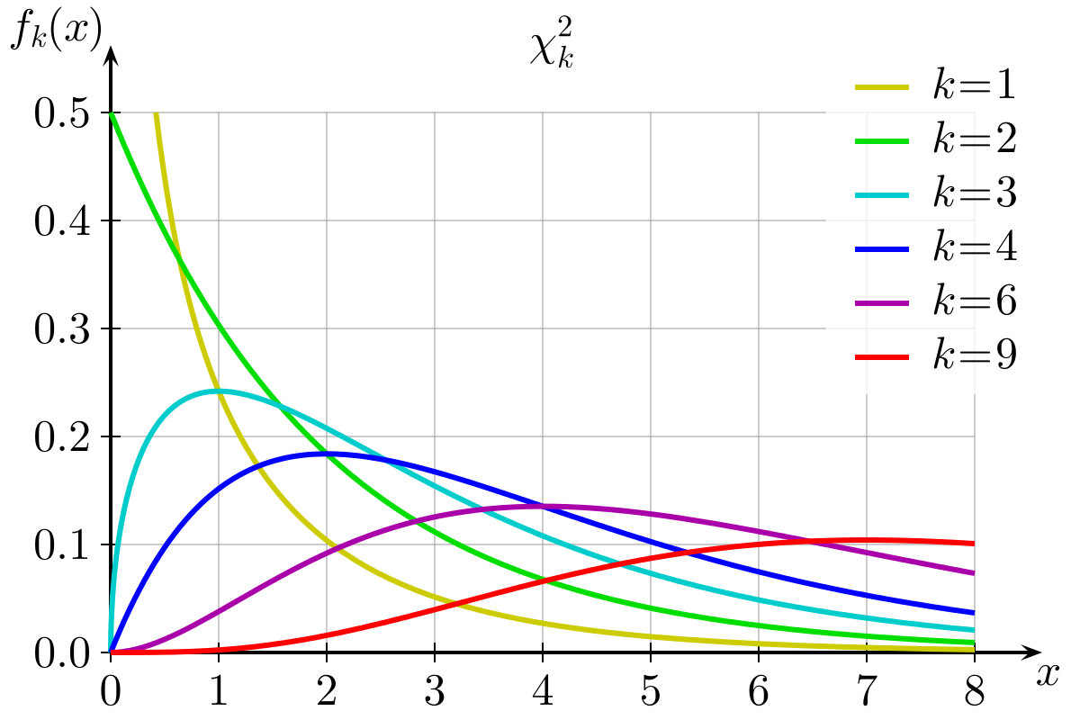
- For the \(\chi^2\) tests, if the null hypothesis is true and there is no difference between the observed and expected frequencies, then our \(\chi^2\)-statistics will follow the \(\chi^2\) distribution (i.e., with 2 categories, most of them will be between 0 and 2, with fewer falling >2, see the yellow line in Figure 1).
- For the \(t\)-tests, if the null hypothesis is true (there is no difference between group means/between our observed mean and some value), then our \(t\)-statistics (if we could do our study loads of times) will mainly fall around 0, and follow a \(t\)-distribution. The precise \(t\)-distribution depends on the degrees of freedom, which in turn depends on how much data we have.
Step 2. We calculate our statistic from our observed data.
Step 3. We ask what the probability is of getting a statistic at least as extreme as we get from Step 2, assuming the null hypothesis we stated in Step 1.
If you’re finding the programming easy, but the statistical concepts difficult
Another way which might help to think about this is that if we can make a computer do something over and over again, we can do stats! You may already be familiar with this idea from exercises with the function replicate()!
- make the computer generate random data, based on some null hypothesis. Do it lots of times.

- what proportion of the simulations produce results similar to the observed data (i.e., as extreme or more extreme)? This is \(p\). The only difference between this and “statistics” is that we calculate \(p\) using math, rather than having to generate random data.
Statistical vs Practical Significance
Let’s suppose that an agricultural company is testing out a new fertiliser they have developed to improve tomato growth. They know that, on average, for every 5cm taller a tomato plant is, it tends to provide 1 more tomato. Taller plants = more tomatoes.
They plant 1000 seeds (taken from the same tomato plant) in the same compost and place them in positions with the same amount of sunlight. 500 of the plants receive 100ml of water daily, and the other 500 receive a 100ml of the fertiliser mixed with water. After 100 days, they measure the height of all the tomato plants (in cm).

You can find the data at https://uoepsy.github.io/data/tomatogrowth.csv.
We want to conduct the appropriate test to determine whether the fertiliser provides a statistically significant improvement to tomato plant growth.
Our outcome variable is growth, which is continuous, and our predictor variable is the grouping (whether they received fertiliser or not). So we’re looking at whether there is a difference in mean growth between the two groups. A t-test will do here.
Our alternative hypothesis is that the difference in means \((treatment - control)\) is greater than 0 (i.e., it improves growth). The t.test() function will use alphabetical ordering of the group variable, so if we say alternative="less" then it is the direction we want \((control - treatment < 0)\):1:
tomato <- read_csv("https://uoepsy.github.io/data/tomatogrowth.csv")
t.test(tomato$height ~ tomato$group, alternative = "less")
    Welch Two Sample t-test

data:  tomato$height by tomato$group
t = -2.0085, df = 997.97, p-value = 0.02243
alternative hypothesis: true difference in means between group control and group treatment is less than 0
95 percent confidence interval:
       -Inf -0.2296311
sample estimates:
  mean in group control mean in group treatment
               115.1955                116.4692
Hooray, it is significant! So should we use this fertiliser on all our tomatoes? We need to carefully consider the agricultural company’s situation: given that the fertiliser is comparitively pricey for them to manufacture, is it worth putting into production?
While the fertiliser does improve plant growth to a statistically significant (at \(\alpha=0.05\)) degree, the improvement is minimal. The difference in means is only 1.2737cm. Will this result in many more tomatoes? Probably not.
Furthermore, if we take a look at the confidence interval provided by the t.test() function, we can see that a plausible value for the true difference in means is 0.23cm, which is tiny!
Further Thoughts
The above example is just a silly demonstration that whether or not our p-value is below some set criteria (e.g., .05, .01, .001) is only a small part of the picture. There are many things which are good to remember about p-values:
With a big enough sample size, even a tiny tiny effect is detectable at <.05. For example, you might be interested in testing if the difference in population means across two groups is 0 (\(\mu_1 - \mu_2 = 0\). Your calculated sample difference could be \(\bar{x}_1 - \bar{x}_2 = 0.00002\) but with a very small p-value of 0.00000001. This would tell you that there is strong evidence that the observed difference in means (0.00002) is significantly different from 0. However, the practical difference, that is - the magnitude of the distance between 0.00002 and 0 - is negligible and of pretty much no interest to practitioners. This is the idea we saw in the tomato-plant example.
The criteria (\(\alpha\)) which we set (at .05, .01, etc.), is arbitrary.
Two things need to be kept in mind: there is the true status of the world (which is unknown to us) and the collected data (which are available and reveal the truth only in part).
An observed p-value smaller than the chosen alpha does not imply the true presence of an effect. The observed difference might be due to sampling variability.
Even if a null hypothesis about the population is actually true, then 5% (if \(\alpha\) = 0.05) of the test-statistics computed on different samples from that population would result in a p-value <.05. If you were to obtain 100 random samples from that population, five out of the 100 p-values are likely to be <.05 even if the null hypothesis about the population was actually true.
If you have a single dataset, and you perform several tests of hypotheses on those data, each test comes with a probability of incorrectly rejecting the null (making a type I error) of 5%. Hence, considering the entire family of tests computed, your overall type I error probability will be larger than 5%. In simple words, this means that if you perform enough tests on the same data, you’re almost sure to reject one of the null hypotheses by mistake. This concept is known as multiple comparisons.
Further Reading (Optional)
There are many different competing approaches to doing statistical analyses.
In this course we are learning about what is known as the frequentist framework. Roughly speaking, this is where probabilities are defined as “long-run frequencies” (i.e., the probability of \(x\) happening over many many trials2). Even within the frequentist approach, there are different views as to how to how this definition of probability is best utilised.
The following links provide some introductory readings to some of the different schools of thought:
The correctly-used p value needs an effect size and CI - don’t worry too much about the background of this blog, but it offers some useful visualisations to show how important it is to remember about the uncertainty in our estimates.