Exercises: Covariance, Correlation & Linear Regression

Covariance & Correlation

Question 0

Go to http://guessthecorrelation.com/ and play the “guess the correlation” game for a little while to get an idea of what different strengths and directions of \(r\) can look like.

Sleepy time

Data: Sleep levels and daytime functioning

A researcher is interested in the relationship between hours slept per night and self-rated effects of sleep on daytime functioning. She recruited 50 healthy adults, and collected data on the Total Sleep Time (TST) over the course of a seven day period via sleep-tracking devices.
At the end of the seven day period, participants completed a Daytime Functioning (DTF) questionnaire. This involved participants rating their agreement with ten statements (see Table 1). Agreement was measured on a scale from 1-5. An overall score of daytime functioning can be calculated by:

1. reversing the scores for items 4,5 and 6 (because those items reflect agreement with positive statements, whereas the other ones are agreement with negative statement);
2. summing the scores on each item; and
3. subtracting the sum score from 50 (the max possible score). This will make higher scores reflect better perceived daytime functioning.

The data is available at https://uoepsy.github.io/data/sleepdtf.csv.

Table 1:

Daytime Functioning Questionnaire

Item	Statement
Item_1	I often felt an inability to concentrate
Item_2	I frequently forgot things
Item_3	I found thinking clearly required a lot of effort
Item_4	I often felt happy
Item_5	I had lots of energy
Item_6	I worked efficiently
Item_7	I often felt irritable
Item_8	I often felt stressed
Item_9	I often felt sleepy
Item_10	I often felt fatigued

Question 1

Load the required libraries (probably just tidyverse for now), and read in the data.
Calculate the overall daytime functioning score, following the criteria outlined above, and make this a new column in your dataset.

Hints

To reverse items 4, 5 and 6, we we need to make all the scores of 1 become 5, scores of 2 become 4, and so on… What number satisfies all of these equations: ? - 5 = 1, ? - 4 = 2, ? - 3 = 3?

To quickly sum across rows, you might find the rowSums() function useful (you don’t have to use it though)
If my items were in columns between 4 to 15:

dataframe$sumscore = rowSums(dataframe[, 4:15])

sleepdtf <- read_csv("https://uoepsy.github.io/data/sleepdtf.csv")
summary(sleepdtf)

      TST             item_1         item_2         item_3         item_4    
 Min.   : 4.900   Min.   :1.00   Min.   :1.00   Min.   :1.00   Min.   :1.00  
 1st Qu.: 7.225   1st Qu.:1.00   1st Qu.:2.00   1st Qu.:1.25   1st Qu.:1.00  
 Median : 7.900   Median :1.00   Median :2.00   Median :2.00   Median :1.00  
 Mean   : 8.004   Mean   :1.58   Mean   :2.46   Mean   :2.38   Mean   :1.26  
 3rd Qu.: 9.025   3rd Qu.:2.00   3rd Qu.:3.00   3rd Qu.:3.00   3rd Qu.:1.00  
 Max.   :11.200   Max.   :3.00   Max.   :5.00   Max.   :5.00   Max.   :3.00  
     item_5         item_6         item_7         item_8        item_9    
 Min.   :1.00   Min.   :1.00   Min.   :1.00   Min.   :1.0   Min.   :1.00  
 1st Qu.:2.00   1st Qu.:2.00   1st Qu.:1.00   1st Qu.:2.0   1st Qu.:2.00  
 Median :2.00   Median :3.00   Median :2.00   Median :2.5   Median :3.00  
 Mean   :2.36   Mean   :2.78   Mean   :2.04   Mean   :2.5   Mean   :2.96  
 3rd Qu.:3.00   3rd Qu.:4.00   3rd Qu.:3.00   3rd Qu.:3.0   3rd Qu.:4.00  
 Max.   :4.00   Max.   :5.00   Max.   :4.00   Max.   :4.0   Max.   :5.00  
    item_10    
 Min.   :1.00  
 1st Qu.:2.00  
 Median :3.00  
 Mean   :2.54  
 3rd Qu.:3.00  
 Max.   :5.00  

To reverse the items, we can simply do 6 minus the score:

sleepdtf <- 
  sleepdtf |> mutate(
    item_4=6-item_4,
    item_5=6-item_5,
    item_6=6-item_6
  ) 

Now we can use rowSums(), and subtract the sum scores from from 50 (the max score):

sleepdtf$dtf = 50-rowSums(sleepdtf[, 2:11])

An alternative way to do this would be:

sleepdtf |> 
  mutate(
    dtf = 50 - (item_1 + item_2 + item_3 + item_4 + item_5 + item_6 + item_7 + item_8 + item_9 + item_10)
  )

Question 2

Calculate the correlation between the total sleep time (TST) and the overall daytime functioning score calculated in the previous question.
Conduct a test to establish the probability of observing a correlation this strong in a sample of this size assuming the true correlation to be 0.

Write a sentence or two summarising the results.

Hints

You can do this all with one function, see 5A #correlation-test.

cor.test(sleepdtf$TST, sleepdtf$dtf)

    Pearson's product-moment correlation

data:  sleepdtf$TST and sleepdtf$dtf
t = 6.244, df = 48, p-value = 1.062e-07
alternative hypothesis: true correlation is not equal to 0
95 percent confidence interval:
 0.4807039 0.7989417
sample estimates:
      cor 
0.6694741 

There was a strong positive correlation between total sleep time and self-reported daytime functioning score (\(r\) = 0.67, \(t(48)\) = 6.24, \(p < .001\)) in the current sample. As total sleep time increased, levels of self-reported daytime functioning increased.

Question 3 (open-ended)

Think about this relationship in terms of causation.

Claim: Less sleep causes poorer daytime functioning.

Why might it be inappropriate to make the claim above based on these data alone? Think about what sort of study could provide stronger evidence for such a claim.

Things to think about:

• comparison groups.
  
• random allocation.
  
• measures of daytime functioning.
  
• measures of sleep time.
  
• other (unmeasured) explanatory variables.

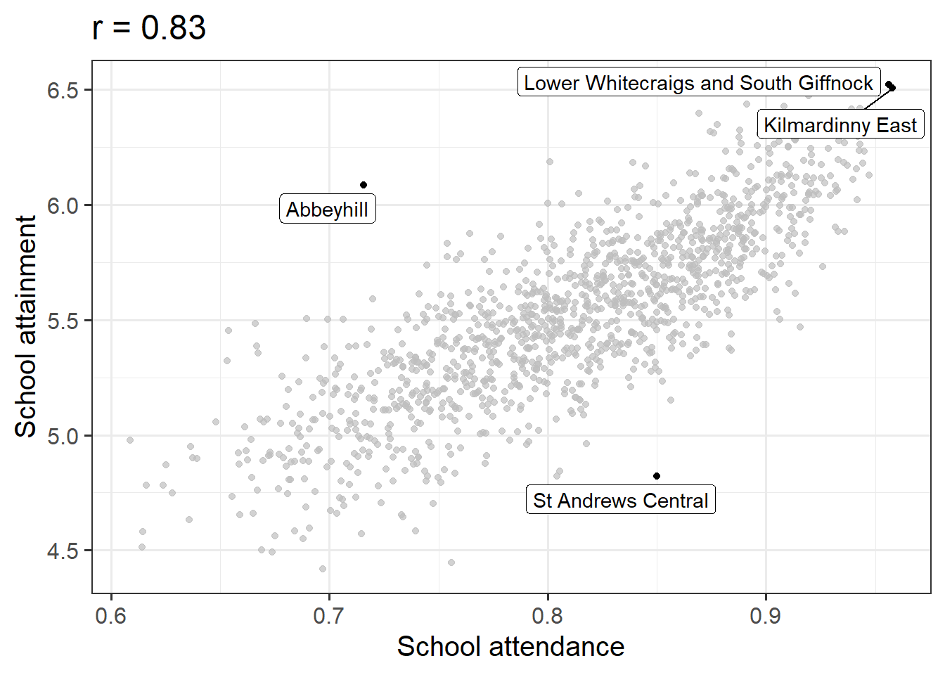
Attendance and Attainment

Data: Education SIMD Indicators

The Scottish Government regularly collates data across a wide range of societal, geographic, and health indicators for every “datazone” (small area) in Scotland.

The dataset at https://uoepsy.github.io/data/simd20_educ.csv contains some of the education indicators (see Table 2).

Table 2:

Education indicators from the 2020 SIMD data

variable	description
intermediate_zone	Areas of scotland containing populations of between 2.5k-6k household residents
attendance	Average School pupil attendance
attainment	Average attainment score of School leavers (based on Scottish Credit and Qualifications Framework (SCQF))
university	Proportion of 17-21 year olds entering university

Question 4

Conduct a test of whether there is a correlation between school attendance and school attainment in Scotland.

Present and write up the results.

Hints

The readings have not included an example write-up for you to follow. Try to follow the logic of those for t-tests and \(\chi^2\)-tests.

• describe the relevant data
• explain what test was conducted and why
• present the relevant statistic, degrees of freedom (if applicable), statement on p-value, etc.
• state the conclusion.

Be careful figuring out how many observations your test is conducted on. cor.test() includes only the complete observations.

simd <- read_csv("https://uoepsy.github.io/data/simd20_educ.csv")

Here are the means of the two variables. We should remember that these calculations will include some observations which have missing data on the other variable.

simd |> 
  summarise(
    m_attendance = mean(attendance, na.rm = TRUE),
    m_attainment = mean(attainment, na.rm = TRUE)
)

# A tibble: 1 × 2
  m_attendance m_attainment
         <dbl>        <dbl>
1        0.811         5.53

Instead, to match with out analysis, we might be inclined to filter our data to complete data:

simd_comp <- simd |> 
  filter(!is.na(attendance) & !is.na(attainment))

simd_comp |>
  summarise(
    m_attendance = mean(attendance),
    m_attainment = mean(attainment),
    sd_attendance = sd(attendance),
    sd_attainment = sd(attainment)
)

# A tibble: 1 × 4
  m_attendance m_attainment sd_attendance sd_attainment
         <dbl>        <dbl>         <dbl>         <dbl>
1        0.811         5.53        0.0696         0.386

cor.test(simd_comp$attendance, simd_comp$attainment)

    Pearson's product-moment correlation

data:  simd_comp$attendance and simd_comp$attainment
t = 51.495, df = 1242, p-value < 2.2e-16
alternative hypothesis: true correlation is not equal to 0
95 percent confidence interval:
 0.8066637 0.8421951
sample estimates:
      cor 
0.8252442 

A correlation test was conducted to assess whether there is a relationship between an area’s average school attendance, and its average school attainment level. A total of 1244 geographical areas were included in the analysis, with a mean school attendance of 0.81 (SD = 0.07) and a mean school attainment score of 5.53 (SD = 0.39).
There was a strong positive correlation between a geographical area’s level of school attendance and its school attainment (\(r\) = 0.83, \(t(1242\) = 51.5, \(p < 0.001\)). We therefore reject the null hypothesis that there is no correlation between an area’s school attendance and attainment. Figure 1 provides a visualisation of the relationship.

Code

ggplot(simd_comp, aes(x=attendance, y=attainment)) + 
  geom_point() + 
  labs(x = "School attendance",
       y = "School attainment")

Figure 1: Positive relationship between geographical areas’ level of school attendance and school attainment

Optional: some extra plotting bits

Sometimes we may want to highlight certain parts of a plot. We can do that using the gghighlight package, and giving it a set of conditions (like we do for filter()) in order for it to decide which points to highlight.
You can see an example below.
We have also created the title by referring to the cor() function, and ’paste’ing it together to “r =”

library(gghighlight)

ggplot(simd_comp, aes(x=attendance, y=attainment)) + 
  geom_point() + 
  gghighlight( (attainment>6 & attendance<.75) | 
               attendance > .95 | 
               (attendance > .82 & attainment<5),
               label_key = intermediate_zone) + 
  labs(x = "School attendance",
       y = "School attainment",
       title = paste0("r = ",
                       round(
                         cor(simd_comp$attendance,
                                  simd_comp$attainment),
                         2)
                       ))

Simple Linear Regression

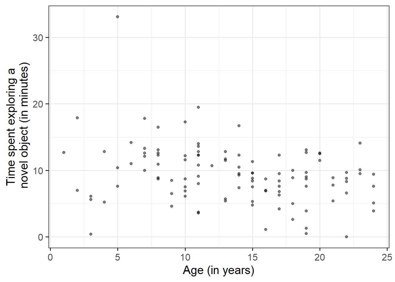
Monkey Exploration

Data: monkeyexplorers.csv

Liu, Hajnosz & Li (2023)¹ have conducted a study on monkeys! They were interested in whether younger monkeys tend to be more inquisitive about new things than older monkeys do. They sampled 108 monkeys ranging from 1 to 24 years old. Each monkey was given a novel object, the researchers recorded the time (in minutes) that each monkey spent exploring the object.

For this week, we’re going to be investigating the research question:

Do older monkeys spend more/less time exploring novel objects?

The data is available at https://uoepsy.github.io/data/monkeyexplorers.csv and contains the variables described in Table 3

Table 3:

Data dictionary for monkeyexplorers.csv

variable	description
name	Monkey Name
age	Age of monkey in years
exploration_time	Time (in minutes) spent exploring the object

Question 5

For this week, we’re going to be investigating the following research question:

Do older monkeys spend more/less time exploring novel objects?

Read in the data to your R session, then visualise and describe the marginal distributions of those variables which are of interest to us. These are the distribution of each variable (time spent exploring, and monkey age) without reference to the values of the other variables.

Hints

• You could use, for example, geom_density() for a density plot or geom_histogram() for a histogram.
• Look at the shape, center and spread of the distribution. Is it symmetric or skewed? Is it unimodal or bimodal?
• Do you notice any extreme observations?

monkeyexp <- read_csv("https://uoepsy.github.io/data/monkeyexplorers.csv")
head(monkeyexp)

# A tibble: 6 × 3
  name            age exploration_time
  <chr>         <dbl>            <dbl>
1 Ed Sheeran        8             13.1
2 Vince Gill       17              6.8
3 Jewel            13             12.8
4 Jaden Smith      18              8.9
5 Reba McEntire    16              1.1
6 Metallica        13              5.7

We can plot the marginal distribution of these two continuous variables as density curves, and add a boxplot underneath to check for the presence of outliers. The width of the geom_boxplot() is always quite wide, so I want to make it narrower so that we can see it at the same time as the density plot. Deciding on the exact value for the width here is just trial and error:

library(patchwork)
# the patchwork library allows us to combine plots together
ggplot(data = monkeyexp, aes(x = age)) +
  geom_density() +
  geom_boxplot(width = 1/300) +
  labs(x = "Age (in years)", 
       y = "Probability density") +

ggplot(data = monkeyexp, aes(x = exploration_time)) +
  geom_density() +
  geom_boxplot(width = 1/175) +
  labs(x = "Time spent exploring a\n novel object (in minutes)", 
       y = "Probability density")

Figure 2: Density plot and boxplot of monkey’s age and their time spent exploring novel objects

The plots suggests that the distributions of monkeys’ ages and the time they spend exploring novel objects are both unimodal. Most of the monkeys are between roughly 8 and 18 years old, and most of them spent between 7 and 12 minutes exploring the objects. The boxplots suggest an outlier in the distribution of exploration-times, with one monkeys spending more than \(1.5 \times IQR\) beyond the 3rd quartile.

To further summarize a distribution, it is typical to compute and report numerical summary statistics such as the mean and standard deviation.

As we have seen, in earlier weeks, one way to compute these values is to use the summarise()/summarize() function from the tidyverse library:

monkeyexp |> 
  summarize(
    mean_age = mean(age), 
    sd_age = sd(age),
    mean_exptime = mean(exploration_time),
    sd_exptime = sd(exploration_time)
    )

# A tibble: 1 × 4
  mean_age sd_age mean_exptime sd_exptime
     <dbl>  <dbl>        <dbl>      <dbl>
1     13.5   5.92         9.40       4.50

The marginal distribution of age is unimodal with a mean of 13.5 years, and a standard deviation of 5.9.
The marginal distribution of time-spent-exploring is unimodal with a mean of 9.4 years, and a standard deviation of 4.5.

Question 6

After we’ve looked at the marginal distributions of the variables of interest in the analysis, we typically move on to examining relationships between the variables.

Visualise and describe the relationship between age and exploration-time among the monkeys in the sample.

Hints

Think about:

• Direction of association
• Form of association (can it be summarised well with a straight line?)
  
• Strength of association (how closely do points fall to a recognizable pattern such as a line?)
• Unusual observations that do not fit the pattern of the rest of the observations and which are worth examining in more detail.
  

Because we are investigating how time-spent-exploring varies with monkeys’ ages, the exploration-time here is the dependent variable (on the y-axis), and age is the independent variable (on the x-axis).

ggplot(data = monkeyexp, aes(x = age, y = exploration_time)) +
  geom_point(alpha = 0.5) +
  labs(x = "Age (in years)", 
       y = "Time spent exploring a\n novel object (in minutes)")

Figure 3: The relationship between monkeys’ age and time-spent-exploring.

There appears to be a moderate negative linear relationship between age and exploration time in these monkeys. Older monkeys appear to spend less time, on average, exploring a novel object. The scatterplot does highlight that there is one one young monkey who is behaving a bit weirdly, and spent quite a long time exploring the object!

To comment numerically on the strength of the linear association we might compute the correlation coefficient that we were introduced to in 5A: Covariance & Correlation

monkeyexp |>
  select(age, exploration_time) |>
  cor()

                        age exploration_time
age               1.0000000       -0.2885495
exploration_time -0.2885495        1.0000000

that is, \(r_{\text{age, exploration-time}} = -0.29\)

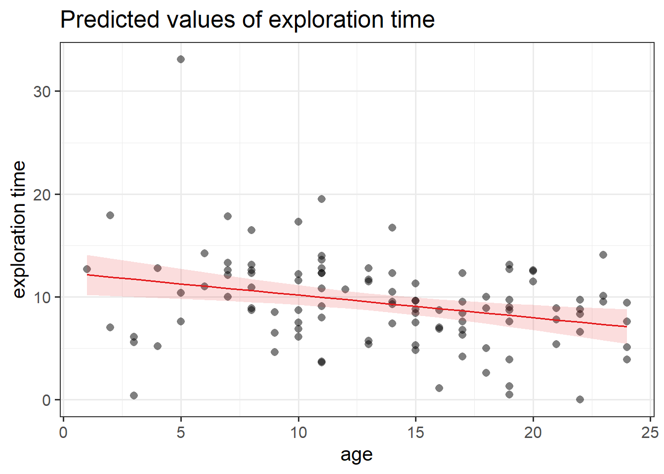
Question 7

Using the lm() function, fit a linear model to the sample data, in which time that monkeys spend exploring novel objects is explained by age. Assign it to a name to store it in your environment.

Hints

You can see how to fit linear models in R using lm() in 5B #fitting-linear-models-in-r

As the variables are in the monkeyexp dataframe, we would write:

model1 <- lm(exploration_time ~ 1 + age, data = monkeyexp)

Question 8

Interpret the estimated intercept and slope in the context of the question of interest.

Hints

We saw how to extract lots of information on our model using summary() (see 5B #model-summary), but there are lots of other functions too.

If we called our linear model object “model1” in the environment, then we can use:

• type model1, i.e. simply invoke the name of the fitted model;
• type model1$coefficients;
• use the coef(model1) function;
• use the coefficients(model1) function;
• use the summary(model1)$coefficients to extract just that part of the summary.

coef(model1)

(Intercept)         age 
   12.36253    -0.21897 

From this, we get that the fitted line is: \[ \widehat{\text{ExplorationTime}} = 12.36 - 0.22 \cdot \text{Age} \\ \]

We can interpret the estimated intercept as:

The estimated average time spent exploring novel objects associated with age of zero is 12.36 minutes.

For the estimated slope we get:

The estimated decrease in average time spent exploring associated with a one year increase in age is -0.22 minutes (or -13 seconds).

Question 9

Test the hypothesis that the population slope is zero — that is, that there is no linear association between exploration time and age in the population.

Hints

You don’t need to do anything for this, you can find all the necessary information in summary() of your model.
See 5B #inference-for-regression-coefficients.

The information is already contained in the row corresponding to the variable “age” in the output of summary(), which reports the t-statistic under t value and the p-value under Pr(>|t|):

summary(model1)

Call:
lm(formula = exploration_time ~ 1 + age, data = monkeyexp)

Residuals:
     Min       1Q   Median       3Q      Max 
-11.3056  -2.3461   0.3841   2.1936  21.8323 

Coefficients:
            Estimate Std. Error t value Pr(>|t|)    
(Intercept) 12.36253    1.04263  11.857  < 2e-16 ***
age         -0.21897    0.07057  -3.103  0.00246 ** 
---
Signif. codes:  0 '***' 0.001 '**' 0.01 '*' 0.05 '.' 0.1 ' ' 1

Residual standard error: 4.324 on 106 degrees of freedom
Multiple R-squared:  0.08326,   Adjusted R-squared:  0.07461 
F-statistic: 9.627 on 1 and 106 DF,  p-value: 0.002458

Recall that very small p-values such as the one for the intercept 2e-16 in the Pr(>|t|) column simply means \(2 \times 10^{-16}\), or 0.0000000000000002. Conventions such as the APA guidelines give rules on how to report these numbers (see, e.g. APA’s number and stats guide). For the p-values in this summary (the one for the intercept and the one for the slope) we could report them as “<.001” and “0.003” respectively.

A significant association was found between age (in years) and time spent exploring novel objects, with exploration time decreasing by on average -0.22 minutes (or -13 seconds) for every additional year of age (\(b = -0.22\), \(SE = 0.071\), \(t(106)=-3.103\), \(p=.003\)).

Question 10

Create a visualisation of the estimated association between age and exploration time.

Hints

There are lots of ways to do this. Check 5B #example, which shows an example of using the sjPlot package to create a plot.

library(sjPlot)
plot_model(model1, type="eff", show.data = TRUE)

$age

Optional: Question 11A

Consider the following:

1. In fitting a linear regression model, we make the assumption that the errors around the line are normally distributed around zero (this is the \(\epsilon \sim N(0, \sigma)\) bit.)
   
2. About 95% of values from a normal distribution fall within two standard deviations of the centre.

We can obtain the estimated standard deviation of the errors (\(\hat \sigma\)) from the fitted model using sigma() and giving it the name of our model.
What does this tell us?

Hints

See 5B #the-error.

The estimated standard deviation of the errors can be obtained by:

sigma(model1)

[1] 4.324399

For any particular age, the time monkeys spend exploring novel objects should be distributed above and below the regression line with standard deviation estimated to be \(\hat \sigma = 4.32\). Since \(2 \hat \sigma = 2 (4.32) = 8.64\), we expect most (about 95%) of the monkeys’ exploration times to be within about 8.6 minutes from the regression line.

Optional: Question 11B

Compute the model-predicted exploration-time for a monkey that is 1 year old.

Hints

Given that you know the intercept and slope, you can calculate this algebraically. However, try to also use the predict() function (see 5B #model-predictions).

Using predict(), we need to give it our model, plus some new data which contains a monkey that has 1 in the age column. First we make a new dataframe with an age variable, with one entry which has the value 1, and then we give that to predict():

age_query <- data.frame(age = c(1))
predict(model1, newdata = age_query)

       1 
12.14356 

Given that our fitted model takes the form:

\[ \widehat{\text{ExplorationTime}} = 12.36 - 0.22 \cdot \text{Age} \]

We are asking what the predicted exploration time is for a monkey with 1 year of age. So we can substitute in “1” for the Age variable: \[ \begin{align} \text{ExplorationTime} &= 12.36 - 0.22 \cdot \text{Age} \\ \text{ExplorationTime} &= 12.36 - 0.22 \cdot 1 \\ \text{ExplorationTime} &= 12.36 - 0.22\\ \text{ExplorationTime} &= 12.14\\ \end{align} \]

Influential Monkeys

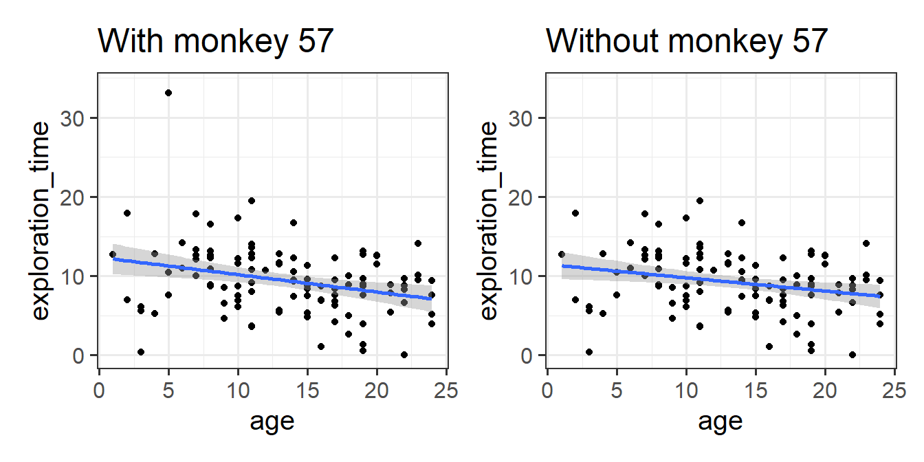
Question 12

Take a look at the assumption plots (see 5B #assumptions) for your model.

• The trick to looking at assumption plots in linear regression is to look for “things that don’t look random”.
• As well as looking for patterns, these plots can also higlight individual datapoints that might be skewing the results. Can you figure out if there are any unusual monkeys in our dataset? Can you re-fit the model without that monkey? When you do so, do your conclusions change?

plot(model1)

From these plots, we can see that the 57th observation is looking a bit influential. It is the one datapoint that is looking weird in all of the plots.
Let’s look at them:

monkeyexp[57, ]

# A tibble: 1 × 3
  name       age exploration_time
  <chr>    <dbl>            <dbl>
1 Lil Fizz     5             33.1

This is a young monkey (5 years old) called “Lil Fizz”, who seems to have spent quite a long time exploring the toy. It’s important to remember that this monkey is a valuable datapoint, despite being a bit different from the general pattern.

However, it would be nice to know how much Lil Fizz is affecting our conclusions, so let’s re-fit the model on everybody except that one monkey

model1a <- lm(exploration_time ~ age, data = monkeyexp[-57, ])
summary(model1a)

Call:
lm(formula = exploration_time ~ age, data = monkeyexp[-57, ])

Residuals:
    Min      1Q  Median      3Q     Max 
-10.558  -2.321   0.427   2.386   9.884 

Coefficients:
            Estimate Std. Error t value Pr(>|t|)    
(Intercept) 11.46135    0.92155  12.437  < 2e-16 ***
age         -0.16781    0.06212  -2.701  0.00805 ** 
---
Signif. codes:  0 '***' 0.001 '**' 0.01 '*' 0.05 '.' 0.1 ' ' 1

Residual standard error: 3.769 on 105 degrees of freedom
Multiple R-squared:  0.06498,   Adjusted R-squared:  0.05608 
F-statistic: 7.297 on 1 and 105 DF,  p-value: 0.008053

Our conclusions haven’t changed - we still have a significant association.

What we have just done is called a “sensitivity analysis” - we’ve asked if our analyses are sensitive to a specific decision we could make (whether or not we include/exclude this monkey).

Code

ggplot(monkeyexp, aes(x=age,y=exploration_time))+
  geom_point()+
  geom_smooth(method=lm, fullrange=TRUE)+
  ylim(0,34) + 
  labs(title="With monkey 57") +

ggplot(monkeyexp[-57,], aes(x=age,y=exploration_time))+
  geom_point()+
  geom_smooth(method=lm, fullrange=TRUE)+
  ylim(0,34) + 
  labs(title="Without monkey 57")

We now have a decision to make. Do we continue with the monkey removed, or do we keep them in? There’s not really a right answer here, but it’s worth noting a practical issue - our assumption plots look considerably better for our model without this monkey.

Whatever we do, when writing up the analysis we need to mention clearly if and why we exclude any observations, and how that decision has/hasn’t influenced our conclusions.

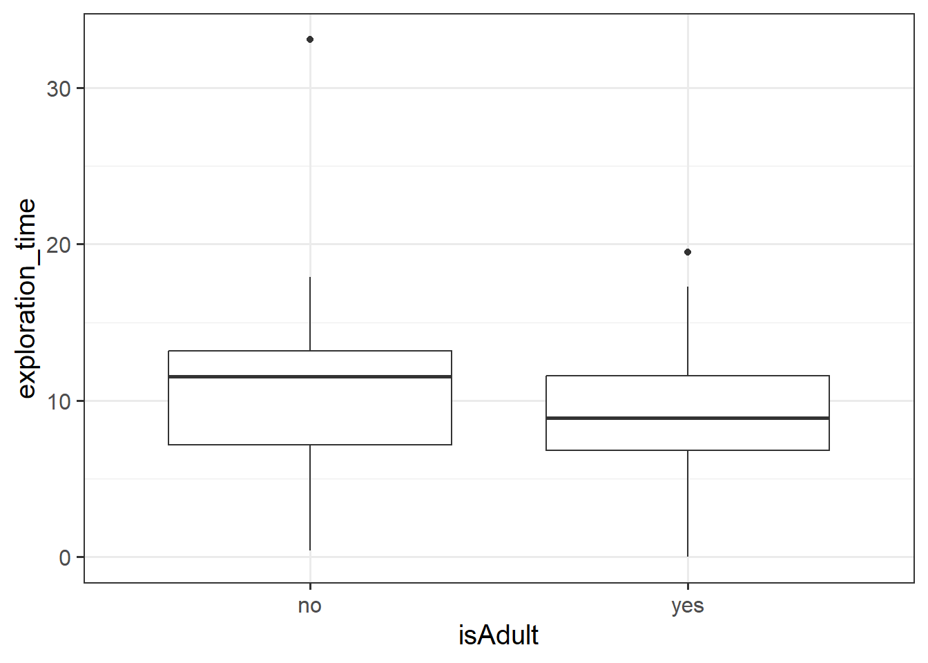
Monkey Exploration in Adulthood

Let’s suppose instead of having measured monkeys’ ages in years, researchers simply recorded whether each monkey was an adult or a juvenile (both Capuchins and Rhesus Macaques reach adulthood at 8 years old).
The code below creates a this new variable for us:

monkeyexp <- monkeyexp |> 
  mutate(
    isAdult = ifelse(age >= 8, "yes","no")
  )

Question 13

Fit the following model, and interpret the coefficients.

\[ \text{ExplorationTime} = b_0 + b_1 \cdot \text{isAdult} + \varepsilon \]

Hints

For help interpreting the coefficients, see 5B #binary-predictors.

model2 <- lm(exploration_time ~ 1 + isAdult, data = monkeyexp)
summary(model2)

Call:
lm(formula = exploration_time ~ 1 + isAdult, data = monkeyexp)

Residuals:
     Min       1Q   Median       3Q      Max 
-11.2556  -2.3694  -0.0444   2.5556  21.4444 

Coefficients:
            Estimate Std. Error t value Pr(>|t|)    
(Intercept)   11.656      1.037  11.239   <2e-16 ***
isAdultyes    -2.711      1.136  -2.386   0.0188 *  
---
Signif. codes:  0 '***' 0.001 '**' 0.01 '*' 0.05 '.' 0.1 ' ' 1

Residual standard error: 4.4 on 106 degrees of freedom
Multiple R-squared:  0.05099,   Adjusted R-squared:  0.04204 
F-statistic: 5.695 on 1 and 106 DF,  p-value: 0.01878

• (Intercept) = the estimated exploration time of juvenile monkeys (11.7 minutes)
• isAdultyes = the estimated change in exploration time from juvenile monkeys to adult monkeys (-2.7 minutes)

ggplot(monkeyexp, aes(x = isAdult, y = exploration_time)) +
  geom_boxplot()

Question 14

We’ve actually already seen a way to analyse questions of this sort (“is the average exploration-time different between juveniles and adults?”)

Run the following t-test, and consider the statistic, p value etc. How does it compare to the model in the previous question?

t.test(exploration_time ~ isAdult, data = monkeyexp, var.equal = TRUE)

t.test(exploration_time ~ isAdult, data = monkeyexp, var.equal = TRUE)

    Two Sample t-test

data:  exploration_time by isAdult
t = 2.3865, df = 106, p-value = 0.01878
alternative hypothesis: true difference in means between group no and group yes is not equal to 0
95 percent confidence interval:
 0.4588049 4.9634174
sample estimates:
 mean in group no mean in group yes 
        11.655556          8.944444 

It is identical! the \(t\)-statistics are the same, the p-values are the same, the degrees of freedom. Everything!

The two sample t-test is actually just a special case of the linear model, where we have a numeric outcome variable and a binary predictor!

And… the one-sample t-test is the linear model without any predictors, so just with an intercept.

t.test(monkeyexp$exploration_time, mu = 0)

    One Sample t-test

data:  monkeyexp$exploration_time
t = 21.722, df = 107, p-value < 2.2e-16
alternative hypothesis: true mean is not equal to 0
95 percent confidence interval:
  8.538785 10.253807
sample estimates:
mean of x 
 9.396296 

interceptonly_model <- lm(exploration_time ~ 1, data = monkeyexp)

summary(interceptonly_model)$coefficients

            Estimate Std. Error  t value     Pr(>|t|)
(Intercept) 9.396296  0.4325657 21.72224 5.060938e-41

Extra! A team task!

Question EXTRA!

The data from this year’s survey that you filled out in the first couple of weeks is available at https://uoepsy.github.io/data/usmr2023.csv.

• Step 1: Using the USMR 2023 survey data, make either the prettiest plot you can or the ugliest plot you can .
• Step 2: Submit your plot! Go to https://forms.office.com/e/KiGevk6xH3 and upload your plot and the code used to create it (save the plot via the plot window in R/take a screenshot/put it in a .Rmd and knit/whatever gets the picture uploaded!)

All plots submitted by end-of-day on 25th October will be rated by a number of non-USMR staff, and prizes made of chocolate will be awarded to the team with the prettiest plot and to the team with the ugliest plot.

Footnotes

1. Not a real study!