4A: Chi-Square Tests

This reading:

What are the basic hypothesis tests that we can conduct when we are interested in variables that have categories instead of numbers?
- Tests of the distribution of a single categorical variable
- Tests of the relationship between two categorical variables

Just like we did with the various types of \(t\)-test, we’re going to continue with some more brief explainers of different basic statistical tests. The past few weeks have focused on tests for numeric outcome variables, where we have been concerned with the mean of that variable (e.g. whether that mean is different from some specific value, or whether it is different between two groups). We now turn to investigate tests for categorical outcome variables.

When studying categorical variables, we tend to be interested in counts (or “frequencies”). These can be presented in tables. With 1 variable, we have a 1 dimensional table.
For example, how many people in the data are left-handed, right-handed, or ambidextrous:

timehands <- read_csv("https://uoepsy.github.io/data/timehands.csv")
table(timehands$handed)


 ambi  left right 
   30   102   870

and with 2 variables, we have a 2-dimensional table (also referred to as a ‘contingency table’). For instance, splitting up those left/right/ambidextrous groups across whether they prefer the morning or night:

table(timehands$handed, timehands$ampm)

       
        morning night
  ambi        6    24
  left       81    21
  right     435   435

We can perform tests to examine things such as:

how likely we are to see our sample frequencies in a single categorical variable, if some some hypothesised null distribution were true (e.g. how likely are we to see the numbers of left/right/ambi people in our sample if in bigger population we expect a 1/3 chance of each?)
how likely we are to see our sample frequencies across two categorical variables, if these variables are independent in the population. (e.g. how likely are we to see the counts in the 2x2 table above, if being left/right/ambi has nothing to do with whether you are a morning or night person).

The test-statistics for these tests (denoted \(\chi^2\), spelled chi-square, pronounced “kai-square”) are obtained by adding up the standardized squared deviations in each cell of a table of frequencies:

\[ \chi^2 = \sum_{all\ cells} \frac{(\text{Observed} - \text{Expected})^2}{\text{Expected}} \] where:

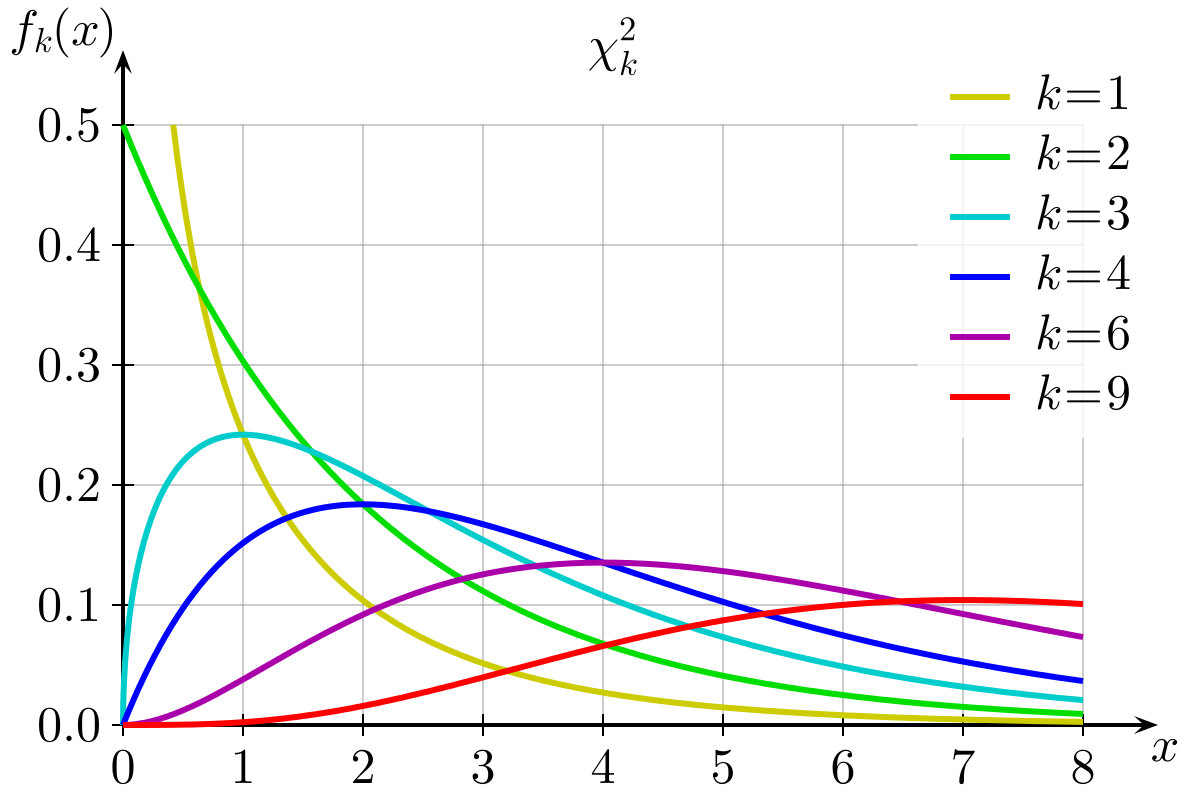
\(\text{Observed}\) = observed count for a cell
\(\text{Expected}\) = expected count for a cell

Just like the \(t\)-statistics we calculate follow \(t\)-distributions, the \(\chi^2\)-statistics follow \(\chi^2\) distributions! If you look carefully at the formula above, it can never be negative (because the value on top of the fraction is squared, and so is always positive). For a given cell of the table, if we observe exactly what we expect, then \(\text{(Observed - Expected)}^2\) becomes zero. The further away the observed count is from the expected count, the larger it becomes.

This means that under the null hypothesis, larger values are less likely. And the shape of our \(\chi^2\) distributions follow this logic. They have higher probability for small values, getting progressively less likely for large values. \(\chi^2\)-distributions also have a degrees of freedom, because with more cells in a table, there are more chances for random deviations between “observed and expected” to come in, meaning we are more likely to see higher test statistics when we have more cells in the table (and therefore more degrees of freedom). You can see the distribution of \(\chi^2\) statistics with different degrees of freedom in Figure 1 below.

\(\chi^2\) Goodness of Fit Test

Purpose

The \(\chi^2\) Goodness of Fit Test is typically used to investigate whether observed sample proportions are consistent with an hypothesis about the proportional breakdown of the various categories in the population.

Examples:
- Do 20% of the adult population suffer from some form of depression?
- Are people equally likely to be born on any of the seven days of the week?
- Are 25% of Smarties brown?
- Are 2/3 of people ‘dog people’ and 1/3 of people ‘cat people’?

Assumptions

Data should be randomly sampled from the population.
Data should be at the categorical or nominal level - goodness-of-fit test is not appropriate for continuous level data.
Expected counts should be at least 5.

Research Question & Data

Research Question: Have proportions of adults suffering no/mild/moderate/severe depression changed from 2019?

In 2019, it was reported that 80% of adults (18+) experienced no symptoms of depression, 12% experienced mild symptoms, 4% experienced moderate symptoms, and 4% experienced severe symptoms.
The dataset is accessible at https://uoepsy.github.io/data/usmr_chisqdep.csv contains data from 1000 people to whom the PHQ-9 depression scale was administered in 2022.

depdata <- read_csv("https://uoepsy.github.io/data/usmr_chisqdep.csv") 
head(depdata)

# A tibble: 6 × 3
  id    dep    fam_hist
  <chr> <chr>  <chr>   
1 ID1   severe n       
2 ID2   mild   n       
3 ID3   no     n       
4 ID4   no     n       
5 ID5   no     n       
6 ID6   no     n

We can see our table of observed counts with the table() function:

table(depdata$dep)


    mild moderate       no   severe 
     143       34      771       52

Quick and easy chisq.test()

We can perform the \(\chi^2\) test very easily, by simply passing the table to the chisq.test() function, and passing it the hypothesised proportions. If we don’t give it any, it will assume they are equal.

Note: the proportions must be in the correct order as the entries in the table!

This will give us the test statistic, degrees of freedom, and the p-value:

# note the order of the table is mild, moderate, no, severe. 
# so we put the proportions in that order
chisq.test(table(depdata$dep), p = c(.12, .04, .8, .04))


    Chi-squared test for given probabilities

data:  table(depdata$dep)
X-squared = 9.9596, df = 3, p-value = 0.01891

If the distribution of no/mild/moderate/severe depression were as suggested (80%/12%/4%/4%), then the probability that we would obtain a test statistic this large (or larger) by random chance alone is .019. With an \(\alpha = 0.05\), we reject the null hypothesis that the proportion of people suffering from different levels of depression are the same as those indicated previously in 2019.

\(\chi^2\) goodness of fit test indicated that the observed proportions of people suffering from no/mild/moderate/severe depression were significantly different (\(\chi^2(3)=9.96, p = .019\)) from those expected under the distribution suggested from a 2019 study (80%/12%/4%/4%).

We can examine where the biggest deviations from the hypothesised distribution are by examining the ‘residuals’:

chisq.test(table(depdata$dep), p = c(.12, .04, .8, .04))$residuals


      mild   moderate         no     severe 
 2.0996031 -0.9486833 -1.0253048  1.8973666

This matches with what we see when we look at the table of counts. With \(n=1000\), under our 2019 distribution, we would expect 800 to have no depression, 120 mild, 40 moderate, and 40 severe.

table(depdata$dep)


    mild moderate       no   severe 
     143       34      771       52

The difference in the moderate “observed - expected” is 6, and the difference in the “no depression” is 29. But these are not comparable, because really the 6 is a much bigger amount of the expected for that category than 29 is for the no depression category. The residuals are a way of standardising these.

They are calculated as: \[ \text{residual} = \frac{\text{observed} - \text{expected}}{\sqrt{expected}} \]

Step-by-step calculations

First we calculate the observed counts:

depdata |> 
  count(dep)

# A tibble: 4 × 2
  dep          n
  <chr>    <int>
1 mild       143
2 moderate    34
3 no         771
4 severe      52

Let’s add to this the expected counts:

depdata |> 
  count(dep) |>
  mutate(
    expected = c(.12, .04, .8, .04)*1000
  )

# A tibble: 4 × 3
  dep          n expected
  <chr>    <int>    <dbl>
1 mild       143      120
2 moderate    34       40
3 no         771      800
4 severe      52       40

How do we measure how far the observed counts are from the expected counts under the null? If we simply subtracted the expected counts from the observed counts and then add them up, you will get 0. Instead, we will square the differences between the observed and expected counts, and then add them up.

One issue, however, remains to be solved. A squared difference between observed and expected counts of 100 has a different weight in these two scenarios:

Scenario 1: \(O = 30\) and \(E = 20\) leads to a squared difference \((O - E)^2 = 10^2 = 100\).
Scenario 2: \(O = 3000\) and \(E = 2990\) leads to a squared difference \((O - E)^2 = 10^2 = 100\)

However, it is clear that a squared difference of 100 in Scenario 1 is much more substantial than a squared difference of 100 in Scenario 2. It is for this reason that we divide the squared differences by the the expected counts to “standardize” the squared deviation.

\[ \chi^2 = \sum_{i} \frac{(\text{Observed}_i - \text{Expected}_i)^2}{\text{Expected}_i} \]

We can calculate each part of the equation:

depdata |> 
  count(dep) |>
  mutate(
    expected = c(.12, .04, .8, .04)*1000,
    sq_diff = (n - expected)^2,
    std_sq_diff = sq_diff/expected
  )

# A tibble: 4 × 5
  dep          n expected sq_diff std_sq_diff
  <chr>    <int>    <dbl>   <dbl>       <dbl>
1 mild       143      120     529        4.41
2 moderate    34       40      36        0.9 
3 no         771      800     841        1.05
4 severe      52       40     144        3.6

The test-statistic \(\chi^2\) is obtained by adding up all the standardized squared deviations:

depdata |> 
  count(dep) |>
  mutate(
    expected = c(.12, .04, .8, .04)*1000,
    sq_diff = (n - expected)^2,
    std_sq_diff = sq_diff/expected
  ) |> 
  summarise(
    chi = sum(std_sq_diff)
  )

# A tibble: 1 × 1
    chi
  <dbl>
1  9.96

The p-value for a \(\chi^2\) Goodness of Fit Test is computed using a \(\chi^2\) distribution with \(df = \text{nr categories} - 1\).
We calculate our p-value by using pchisq() and we have 4 levels of depression, so \(df = 4-1 = 3\).

pchisq(9.959583, df=3, lower.tail=FALSE)

[1] 0.01891284

\(\chi^2\) Test of Independence

Purpose

The \(\chi^2\) Test of Independence is used to determine whether or not there is a significant association between two categorical variables. To examine the independence of two categorical variables, we have a contingency table:

                   Family History of Depression
Depression Severity   n   y
           mild      93  50
           moderate  23  11
           no       532 239
           severe    37  15

Examples:
- Is depression severity associated with having a family history of depression?
- Are people with blue eyes more likely to be over 6 foot tall?
- Are people who carry the APOE-4 gene more likely to have mild cognitive impairment?

Assumptions

Two or more categories (groups) for each variable.
Independence of observations
- there is no relationship between the subjects in each group
Large enough sample size, such that:
- expected frequencies for each cell are at least 1
- expected frequencies should be at least 5 for the majority (80%) of cells

Research Question & Data

Research Question: Is severity of depression associated with having a family history of depression?

The dataset accessible at https://uoepsy.github.io/data/usmr_chisqdep.csv contains data from 1000 people to whom the PHQ-9 depression scale was administered in 2022, and for which respondents were asked a brief family history questionnaire to establish whether they had a family history of depression.

depdata <- read_csv("https://uoepsy.github.io/data/usmr_chisqdep.csv")
head(depdata)

# A tibble: 6 × 3
  id    dep    fam_hist
  <chr> <chr>  <chr>   
1 ID1   severe n       
2 ID2   mild   n       
3 ID3   no     n       
4 ID4   no     n       
5 ID5   no     n       
6 ID6   no     n

We can create our contingency table:

table(depdata$dep, depdata$fam_hist)

          
             n   y
  mild      93  50
  moderate  23  11
  no       532 239
  severe    37  15

And even create a quick and dirty visualisation of this too:

plot(table(depdata$dep, depdata$fam_hist))

Quick and easy chisq.test()

Again, we can perform this test very easily by passing the table to the chisq.test() function. We don’t need to give it any hypothesised proportions here - it will work them out based on the null hypothesis that the two variables are independent.

chisq.test(table(depdata$dep, depdata$fam_hist))


    Pearson's Chi-squared test

data:  table(depdata$dep, depdata$fam_hist)
X-squared = 1.0667, df = 3, p-value = 0.7851

If there was no association between depression severity and having a family history of depression, then the probability that we would obtain a test statistic this large (or larger) by random chance alone is 0.79. With an \(\alpha=.05\), we fail to reject the null hypothesis that there is no association between depression severity and family history of depression.

A \(\chi^2\) test of independence indicated no significant association between severity and family history (\(\chi^2(3)=1.07, p=.785\)), suggesting that a participants’ severity of depression was not dependent on whether or not they had a family history of depression.

We can see the expected and observed counts:

chisq.test(table(depdata$dep, depdata$fam_hist))$expected

          
                 n       y
  mild      97.955  45.045
  moderate  23.290  10.710
  no       528.135 242.865
  severe    35.620  16.380

chisq.test(table(depdata$dep, depdata$fam_hist))$observed

          
             n   y
  mild      93  50
  moderate  23  11
  no       532 239
  severe    37  15

Step-by-step calculations

We have our observed table:

table(depdata$dep, depdata$fam_hist)

          
             n   y
  mild      93  50
  moderate  23  11
  no       532 239
  severe    37  15

To work out our expected counts, we have to do something a bit tricky. Let’s look at the variables independently:

table(depdata$fam_hist)


  n   y 
685 315

table(depdata$dep)


    mild moderate       no   severe 
     143       34      771       52

With \(\frac{315}{315+685} = 0.315\) of the sample having a family history, then if depression severity is independent of family history, we would expect that 0.315 of each severity group to have a family history of depression. For example, for the mild depression, with 143 people, we would expect \(143 \times 0.315 = 45.045\) people in that group to have a family history of depression.

For a given cell of the table we can calculate the expected count as \(\text{row total} \times \frac{\text{column total}}{\text{samplesize}}\).
Or, quickly in R:

obs <- table(depdata$dep, depdata$fam_hist)
exp <- rowSums(obs) %o% colSums(obs) / sum(obs)
exp

               n       y
mild      97.955  45.045
moderate  23.290  10.710
no       528.135 242.865
severe    35.620  16.380

Now that we have our table of observed counts, and our table of expected counts, we can actually fit these into our formula to calculate the test statistic:

sum ( (obs - exp)^2 / exp )

[1] 1.066686

The p-value is computed using a \(\chi^2\) distribution with \(df = (\text{nr rows} - 1) \times (\text{nr columns} - 1)\).

Why is this? Well, remember that the degrees of freedom is the number of values that are free to vary as we estimate parameters. In a table such as the one below, where we have 4 rows and 2 columns, the degrees of freedom is the number of cells in the table that can vary before we can simply calculate the values of the other cells (where we’re constrained by the need to sum to our row/column totals).

We have 4 rows, and 2 columns, so \(df = (4-1) \times (2-1) = 3\).

pchisq(1.066686, df = 3, lower.tail=FALSE)

[1] 0.7851217