Week 8 Exercises: CFA

New packages

Make sure you have these packages installed:

• lavaan
• semPlot

the language of diagrams

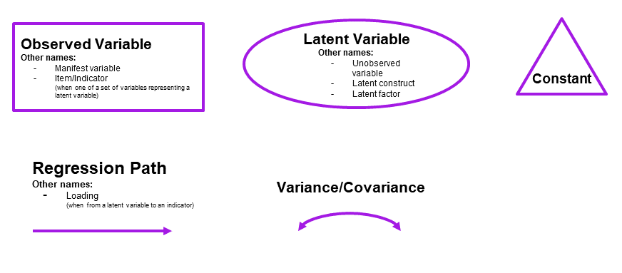
It is common to think about confirmatory factor models (and structural equation models, which we will go on to learn about) in terms of the connections between variables when drawn on a whiteboard (and those that are left undrawn). By representing a theoretical model as paths to and from different variables, we open up a whole new way of thinking about how we model the world around us. These “path diagrams” have different shapes and symbols to denote the covariances, regressions, observed variables and latent variables.

• Observed variables are represented by squares or rectangles. These are the named variables of interest which exist in our dataset - i.e. the ones which we have measured directly.
• Latent variables are represented as ovals/ellipses or circles. These are unobserved variables that we can only reason about and have not (or cannot) directly measured.
  
• Covariances are represented by double-headed arrows. In many diagrams these are curved.
  
• Regressions are shown by single headed arrows (e.g., an arrow from \(x\) to \(y\) for the path \(y \sim x\)). Factor loadings are also regression paths - specifying a factor structure is simply to say that some measured variables \(y_1\,,\, ...\, ,\, y_k\) are each regressed onto some unmeasured factor(s). The formula \(y_1 = \lambda_1 \cdot F + u_1\) looks an awful lot like \(y = b \cdot x + \epsilon\), we just do not observe \(F\)!.

Figure 1: Path/SEM diagrams contain various shapes and symbols to represent different types of variable and the relationships between them.

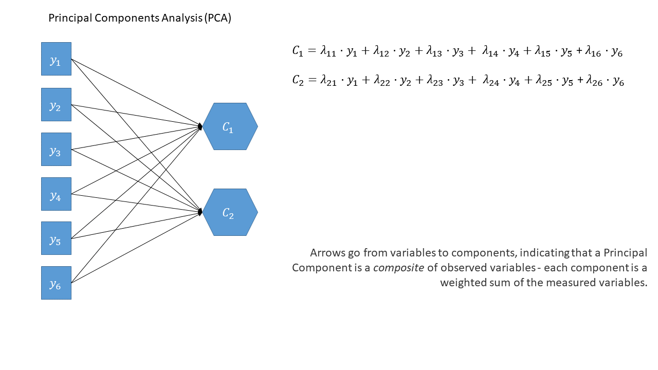
PCA as a diagram

Used for:
Reducing from a lot of correlated variables down to a smaller set of orthogonal (uncorrelated) components that capture a substantial amount of the variance. The components we get out are a bit like “composites” - they are a weighted sum of the original variables, and can be useful in subsequent analyses. For instance, if you have 20 predictors in a linear regression model that are highly correlated with one another (remember multicollinearity?), you might be able to instead use a small number of orthogonal components!

As a diagram
Note that the idea of a ‘composite’ requires us to use a special shape (the hexagon), but many people would just use a square.

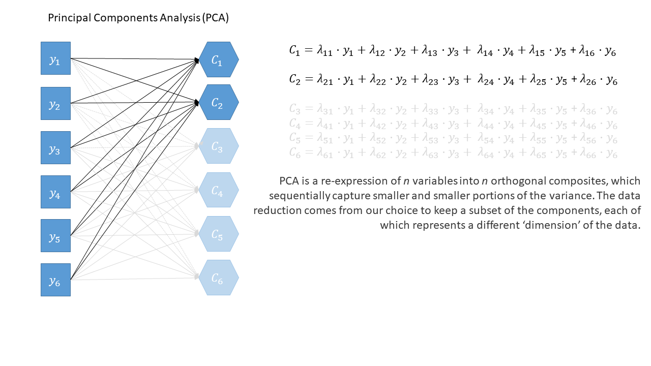
optional: PCA in full

Principal components sequentially capture the orthogonal (i.e., perpendicular) dimensions of the dataset with the most variance. The data reduction comes when we retain fewer components than we have dimensions in our original data. So if we were being pedantic, the diagram for PCA would look something like the diagram below. If the idea of ‘dimensions’ of a dataset is still a bit confusing, you can see a fun 3-dimensional explanation here: PCA in 3D

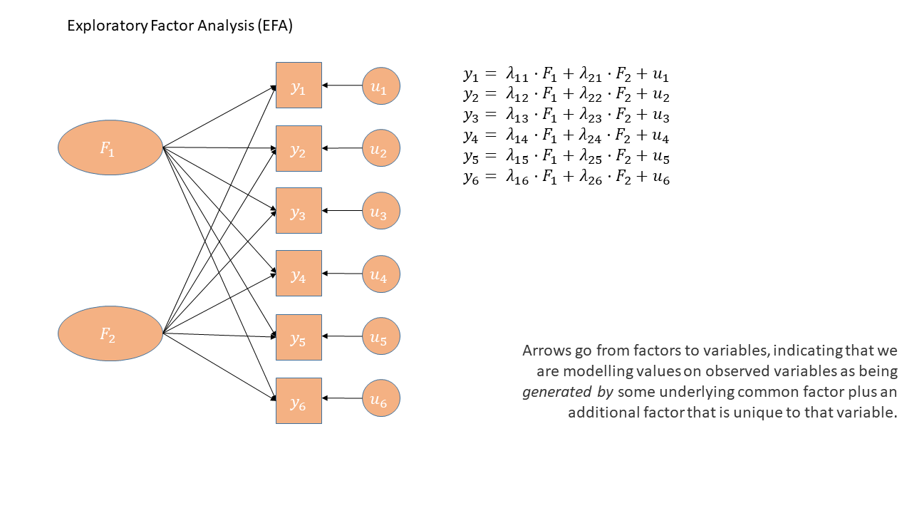
EFA as a diagram

Used for:
EFA is generally used with the aim of understanding the underlying constructs or latent variables that may be driving observed patterns of responses or behaviors. Often used in construction of questionnaires, scale development, and in the initial stages of developing theoretical frameworks.

As a diagram
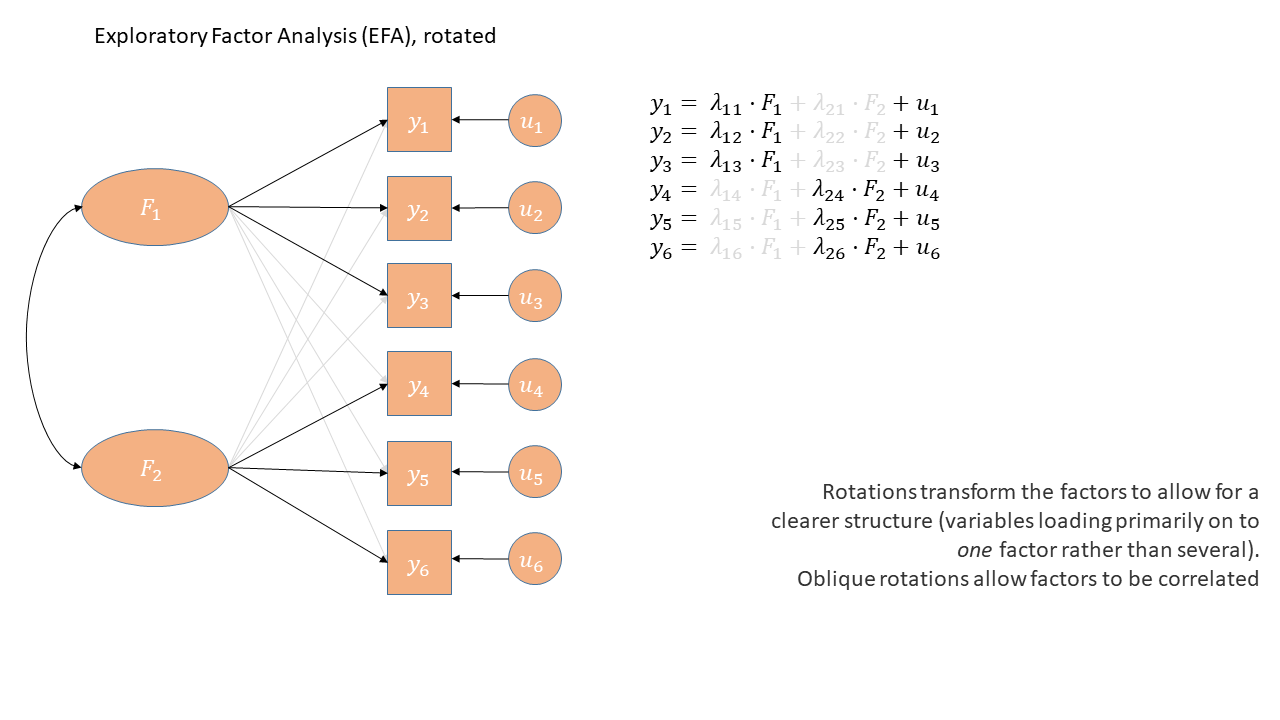
Exploratory Factor Analysis as a diagram has arrows going from the factors to the observed variables. Unlike PCA, we also have ‘uniqueness’ factors for each variable, representing the various stray causes that are specific to each variable. Sometimes, these uniqueness are represented by an arrow only, but they are technically themselves latent variables, and so can be drawn as circles.

When we apply a rotation to an EFA, we make it so that some loadings are smaller and some are higher - essentially creating a ‘simple structure’ (where each variable loads strongly on only one factor and weakly on all other factors). This structure simplifies the interpretation of factors, making them more distinct and easily understandable. With oblique rotations, we also allow factors to be correlated, as indicated by the double headed arrow between them in the diagram below

CFA as a diagram

Used for:
CFA is a method that allows us to assess the validity of a hypothesized factor structure (or to compare competing hypothesized structures). Typically factor structures fitted are ones that have been proposed based on theory or on previous research.

As a diagram
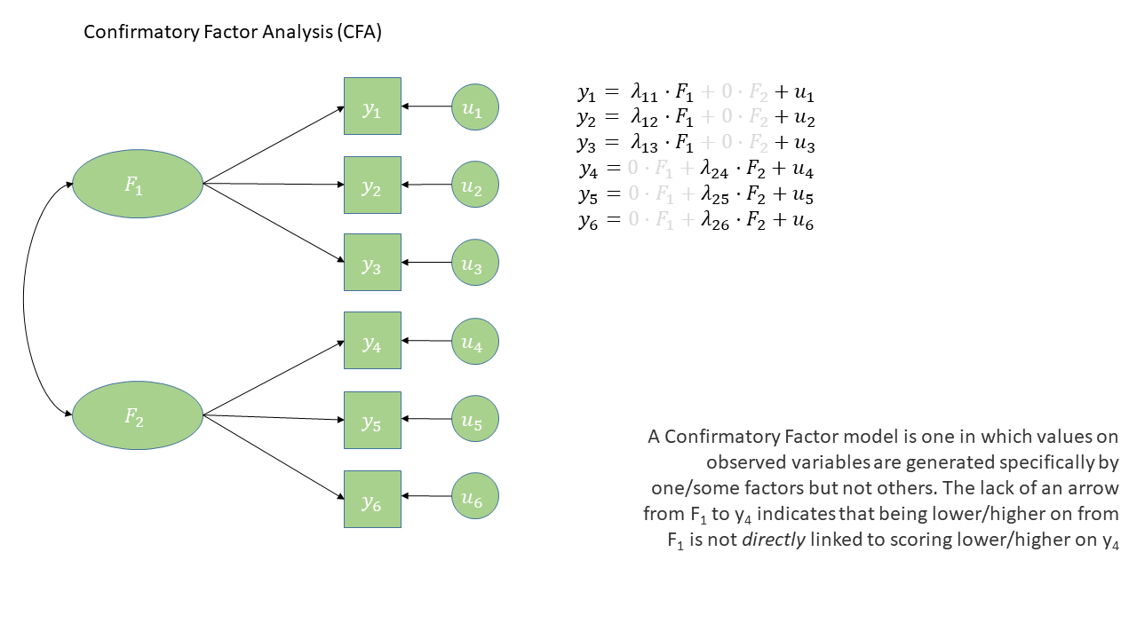
The diagram for a Confirmatory Factor Analysis model looks very similar to that of an exploratory factor analysis, but we now have the explicit absence of some arrows - i.e. a variable loads on to a specific factor (or factors - we can have a variable that loads on multiple), and not on others.

Note that this is a change from the ‘exploratory’ nature of EFA, to a situation in which we are explicitly imposing a theoretical model on the data.

Conduct Problems

Data: conduct_problems_2.csv

Last week we conducted an exploratory factor analysis of a dataset to try and identify an optimal factor structure for a new measure of conduct (i.e., antisocial behavioural) problems.

This week, we’ll conduct some confirmatory factor analyses (CFA) of the same inventory to assess the extent to which this 2-factor structure fits an independent sample. To do this, we have administered our measure to a new sample of n=600 adolescents.

We have re-ordered the questionnaire items to be grouped into the two types of behaviours:

Non-Aggressive Behaviours

item	behaviour
item 1	Stealing
item 2	Lying
item 3	Skipping school
item 4	Vandalism
item 5	Breaking curfew

Aggressive Behaviours

item	behaviour
item 6	Threatening others
item 7	Bullying
item 8	Spreading malicious rumours
item 9	Using a weapon
item 10	Fighting

The data are available as a .csv at https://uoepsy.github.io/data/conduct_problems_2.csv

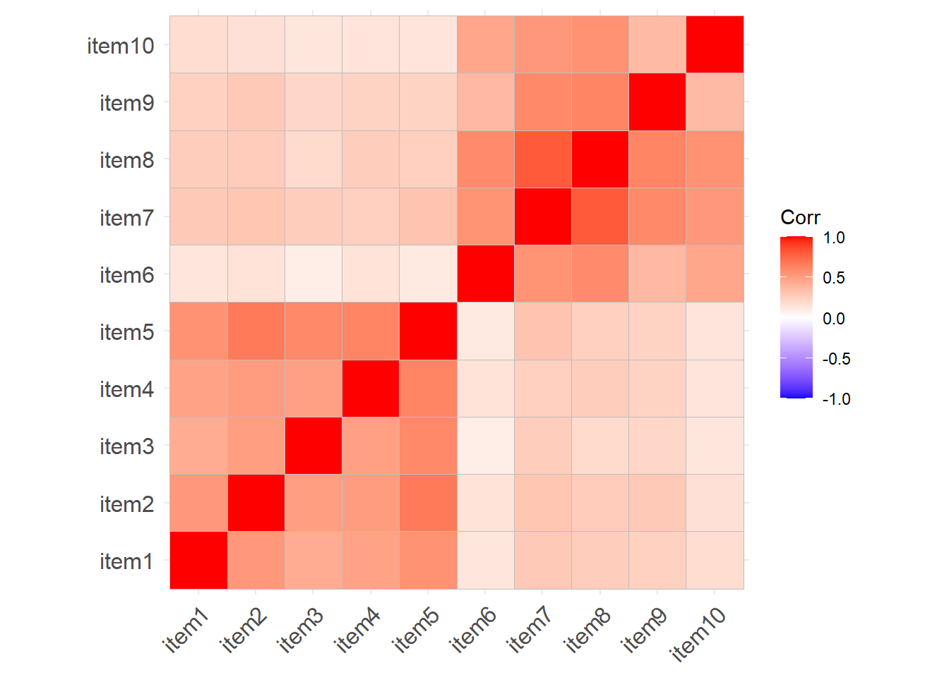
Question 1

Read in the data. Take a look at the correlation matrix.

library(tidyverse)
cp2 <- read_csv("https://uoepsy.github.io/data/conduct_problems_2.csv")

cor(cp2)

           item1     item2      item3     item4     item5      item6     item7
item1  1.0000000 0.5254249 0.43498606 0.4831121 0.5644047 0.13450795 0.2806369
item2  0.5254249 1.0000000 0.50099054 0.5119842 0.6740107 0.15239358 0.3031997
item3  0.4349861 0.5009905 1.00000000 0.4897339 0.5990709 0.09463966 0.2557407
item4  0.4831121 0.5119842 0.48973386 1.0000000 0.6199783 0.14847703 0.2492471
item5  0.5644047 0.6740107 0.59907089 0.6199783 1.0000000 0.11353641 0.3112458
item6  0.1345080 0.1523936 0.09463966 0.1484770 0.1135364 1.00000000 0.5461757
item7  0.2806369 0.3031997 0.25574075 0.2492471 0.3112458 0.54617567 1.0000000
item8  0.2576481 0.2748175 0.19355398 0.2553712 0.2463290 0.59441335 0.8009591
item9  0.2444337 0.2759875 0.20798523 0.2260156 0.2333758 0.36915878 0.5988582
item10 0.1783069 0.1618631 0.12924914 0.1433759 0.1394748 0.46316014 0.5316143
           item8     item9    item10
item1  0.2576481 0.2444337 0.1783069
item2  0.2748175 0.2759875 0.1618631
item3  0.1935540 0.2079852 0.1292491
item4  0.2553712 0.2260156 0.1433759
item5  0.2463290 0.2333758 0.1394748
item6  0.5944133 0.3691588 0.4631601
item7  0.8009591 0.5988582 0.5316143
item8  1.0000000 0.6169829 0.5557168
item9  0.6169829 1.0000000 0.3613253
item10 0.5557168 0.3613253 1.0000000

Just from the visual, it looks like the same factor structure is present in this sample.

library(ggcorrplot)
ggcorrplot(cor(cp2))

Question 2

Fit the proposed 2 factor model in lavaan.

The lavaan package

For the remaining weeks of the course, we’re going to rely heavily on the lavaan (Latent Variable Analysis) package. This is the main package in R for fitting structural equation models, and there is a huge scope of what we can do with it.

Operators in lavaan

The first thing to get to grips with is the various new operators which lavaan allows us to use.

Our standard multiple regression formula in R was specified as

y ~ x1 + x2 + x3 + ...

In lavaan, we continue to fit regressions using the ~ symbol, but we can also specify the construction of latent variables using =~ and residual variances & covariances using ~~.

Formula type	Operator	Mnemonic
latent variable definition	=~	“is measured by”
regression	~	“is regressed on”
(residual) (co)variance	~~	“is correlated with”
intercept	~1	“has an intercept”
defined parameters	:=	“is defined as”

(from https://lavaan.ugent.be/tutorial/syntax1.html)

Fitting models with lavaan

In practice, fitting models in lavaan tends to be a little different from things like lm() and (g)lmer(). Instead of including the model formula inside the fit function (e.g., lm(y ~ x1 + x2, data = df)), we tend to do it in a step-by-step process. This is because as our models become more complex, our formulas can pretty long!

In lavaan, it is typical to write the model as a character string (e.g. model <- "y ~ x1 + x2") and then we pass that formula along with the data to the relevant lavaan function such as cfa() or sem(), giving it the formula and the data: cfa(model, data = mydata).

1. Specify the model:

mymodel <- "
  factor1 =~ item1 + item2 + .....
  factor2 =~ item6 + ...... 
  ...
  ..
"

2. Estimate the model (other fitting functions include sem(), growth() and lavaan()):

myfittedmodel <- cfa(mymodel, data = mydata)

3. Examine the fitted model:

summary(myfittedmodel)

The output of the summary() will show you each estimated parameter in your model. It groups these according to whether they are loadings onto latent variables, covariances, regressions, variances etc.

library(lavaan)
cpmod <- "
  # the non-aggressive problems factor
  nonagg =~ item1 + item2 + item3 + item4 + item5

  # the aggressive problems factor
  agg =~ item6 + item7 + item8 + item9 + item10

  # covariance between the two factors
  # (this is included by default in cfa)
  agg ~~ nonagg
"

cpmod.est <- cfa(cpmod, data = cp2)

summary(cpmod.est)

lavaan 0.6-18 ended normally after 27 iterations

  Estimator                                         ML
  Optimization method                           NLMINB
  Number of model parameters                        21

  Number of observations                           600

Model Test User Model:
                                                      
  Test statistic                                65.765
  Degrees of freedom                                34
  P-value (Chi-square)                           0.001

Parameter Estimates:

  Standard errors                             Standard
  Information                                 Expected
  Information saturated (h1) model          Structured

Latent Variables:
                   Estimate  Std.Err  z-value  P(>|z|)
  nonagg =~                                           
    item1             1.000                           
    item2             1.217    0.076   15.965    0.000
    item3             1.012    0.070   14.424    0.000
    item4             1.146    0.077   14.967    0.000
    item5             1.360    0.078   17.412    0.000
  agg =~                                              
    item6             1.000                           
    item7             1.419    0.082   17.331    0.000
    item8             1.437    0.081   17.662    0.000
    item9             1.093    0.077   14.125    0.000
    item10            0.950    0.073   13.073    0.000

Covariances:
                   Estimate  Std.Err  z-value  P(>|z|)
  nonagg ~~                                           
    agg               0.156    0.023    6.856    0.000

Variances:
                   Estimate  Std.Err  z-value  P(>|z|)
   .item1             0.574    0.037   15.398    0.000
   .item2             0.477    0.035   13.778    0.000
   .item3             0.551    0.036   15.262    0.000
   .item4             0.597    0.040   14.867    0.000
   .item5             0.264    0.028    9.537    0.000
   .item6             0.561    0.035   16.193    0.000
   .item7             0.228    0.021   10.767    0.000
   .item8             0.153    0.019    8.122    0.000
   .item9             0.566    0.035   15.978    0.000
   .item10            0.587    0.036   16.351    0.000
    nonagg            0.453    0.052    8.701    0.000
    agg               0.381    0.045    8.396    0.000

Question 3

Latent variable models like CFA come with a whole bucket load of ‘fit indices’ as metrics of how well our model is reflecting the observed data.

We can get out these indices by either asking for the most common fit indices to be printed inside all of our summary output:

summary(myfittedmodel, fit.measures = TRUE)

Or by asking for all available indices with:

fitmeasures(myfittedmodel)
# to get just a select few, we can index the desired ones:
fitmeasures(myfittedmodel)[c("rmsea","srmr","tli","cfi")]

Examine the fit of the 2-factor model of conduct problems to this new sample of 600 adolescents.

“Model Fit”

You’ll have heard the term “model fit” many times when learning about statistics. However, the exact meaning of the phrase is different for different modelling frameworks.

We can think more generally as “model fit” as asking “how well does our model reproduce the characteristics of the data that we observed?”. In things like multiple regression, this has been tied to the question of “how much variance can we explain in outcome \(y\) with our set of predictors?”¹.

For methods like CFA, path analysis and SEM, we are working with models that run on covariances matrices, so “model fit” becomes “how well can our model reproduce our observed covariance matrix?”.

Degrees of Freedom

In regression, we could only talk about model fit if we had more than 2 datapoints. This is because there is only one possible line that we can fit between 2 datapoints, and this line explains all of the variance in the outcome variable (it uses up all our 2 degrees of freedom to estimate 1) the intercept and 2) the slope).

The logic is the same for model fit in terms of CFA and SEM - we need more degrees of freedom than we have parameters that are estimated.

The difference is that it is all in terms of our covariance matrix, rather than individual observations. The idea is that we need to be estimating fewer paths (e.g. parameters) than there are variances/covariances in our covariance matrix. This is because if we just fit paths between all our variables, then our model would be able to reproduce the data perfectly (just like a regression with 2 datapoints has an \(R^2\) of 1).

The degrees of freedom for methods like CFA, Path and SEM, that are fitted to the covariance matrix of our data, correspond to the number of knowns (observed covariances/variances from our sample) minus the number of unknowns (parameters to be estimated by the model).

• degrees of freedom = number of knowns - number of unknowns
  • number of knowns: how many variances/covariances in our data?
    The number of knowns in a covariance matrix of \(k\) observed variables is equal to \(\frac{k \cdot (k+1)}{2}\).
    
  • number of unknowns: how many parameters is our model estimating?
    We can reduce the number of unknowns (thereby getting back a degree of freedom) by fixing parameters to be specific values. By removing a path altogether, we are fixing it to be zero.

A model is only able to be estimated if it has at least 0 degrees of freedom (if there are as many knowns as unknowns). A model with 0 degrees of freedom is termed just-identified. An under-identified model is one with \(<0\) degrees of freedom, and an over-identified one has \(>0\) degrees of freedom.

Fit Indices

There are loads of different metrics that people use to examine model fit for CFA and SEM, and there’s lots of debate over the various merits and disadvantages as well as the proposed cut-offs to be used with each method.

The most fundamental test of model fit is a \(\chi^2\) test, which reflects the discrepancy between our observed covariance matrix and the model-implied covariance matrix. If we denote the population covariance matrix as \(\Sigma\) and the model-implied covariance matrix as \(\Sigma(\Theta)\), then we can think of the null hypothesis here as \(H_0: \Sigma - \Sigma(\Theta) = 0\). In this way our null hypothesis is that our theoretical model is correct (and can therefore perfectly reproduce the covariance matrix), therefore a significant result indicates poor fit. It is very sensitive to departures from normality, as well as sample size (for models with \(n>400\), the \(\chi^2\) is almost always significant), and can often lead to rejecting otherwise adequate models.

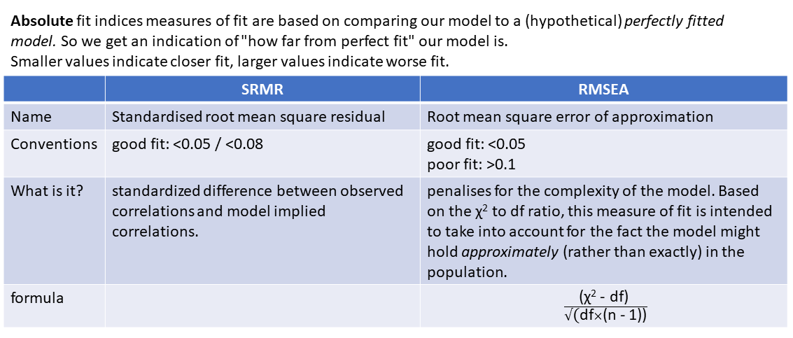
Alongside this, the main four fit indices that are commonly used are known as RMSEA, SRMR, CFI and TLI. Smaller values of RMSEA and SRMR mean better fit while larger values of CFI and TLI mean better fit.

Convention: if \(\textrm{RMSEA} < .05\), \(\textrm{SRMR} < .05\), \(\textrm{TLI} > .95\) and \(\textrm{CFI} > .95\) then the model fits well.

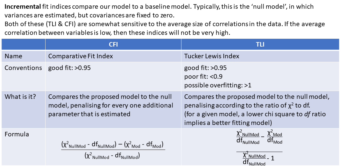
optional: absolute fit indices

optional: incremental fit indices

Our model fits well by all metrics!

fitmeasures(cpmod.est)[c("srmr","rmsea","cfi","tli")]

      srmr      rmsea        cfi        tli 
0.03454489 0.03945991 0.98862263 0.98494172 

Question 4

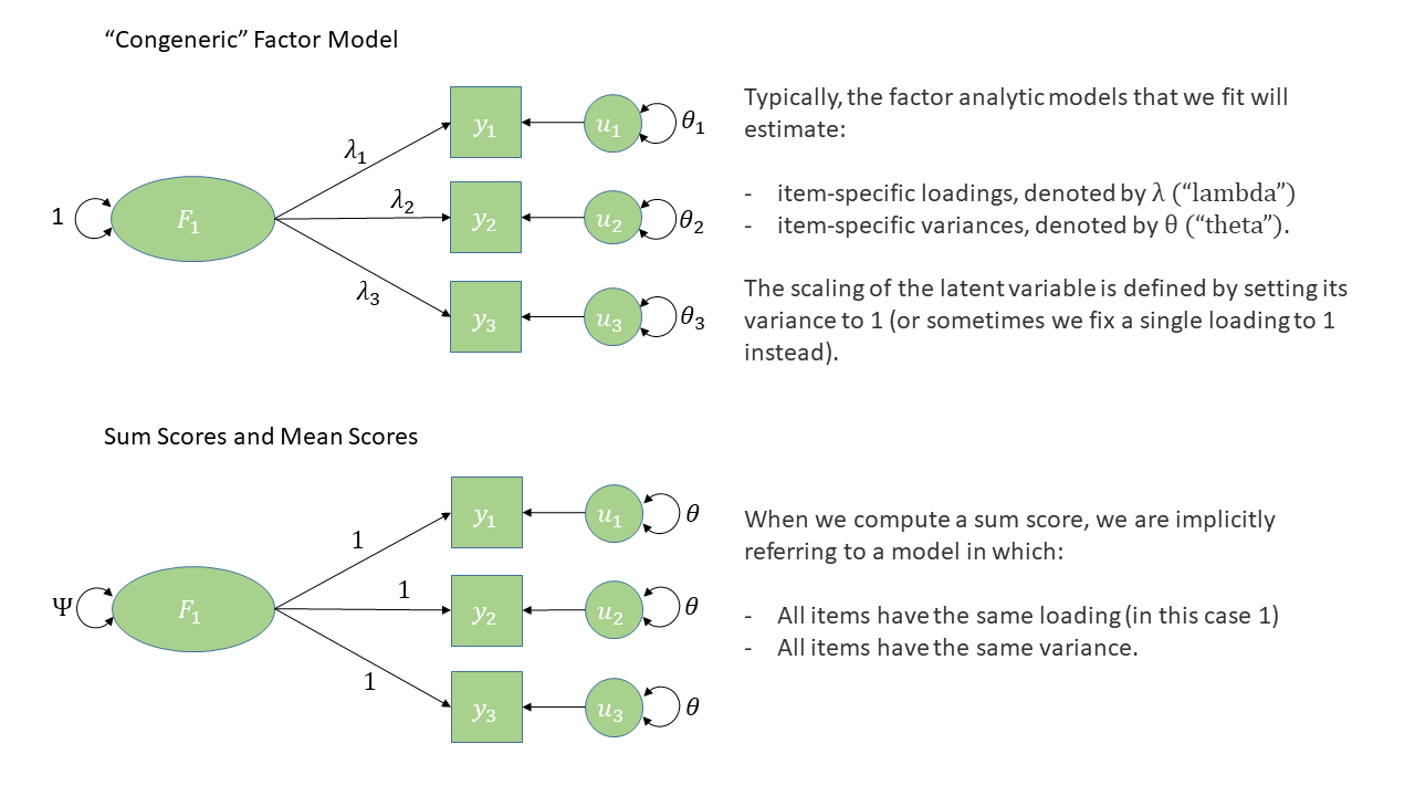
Take a look at the loadings of our variables on to the latent factors (these are in the estimate column under “Latent Variables” in the summary()).

In EFA, our factor loadings were always <1, because they were standardised loadings (where the factor and item were both standardised to have a variance of 1). Because a latent variable is unobserved, it’s actually up to us how we define its scale! In CFA, the default is to make it have the same scale as its first item, which is why the first loading for each factor is exactly 1, and has no standard error associated with it - it’s fixed, rather than estimated.

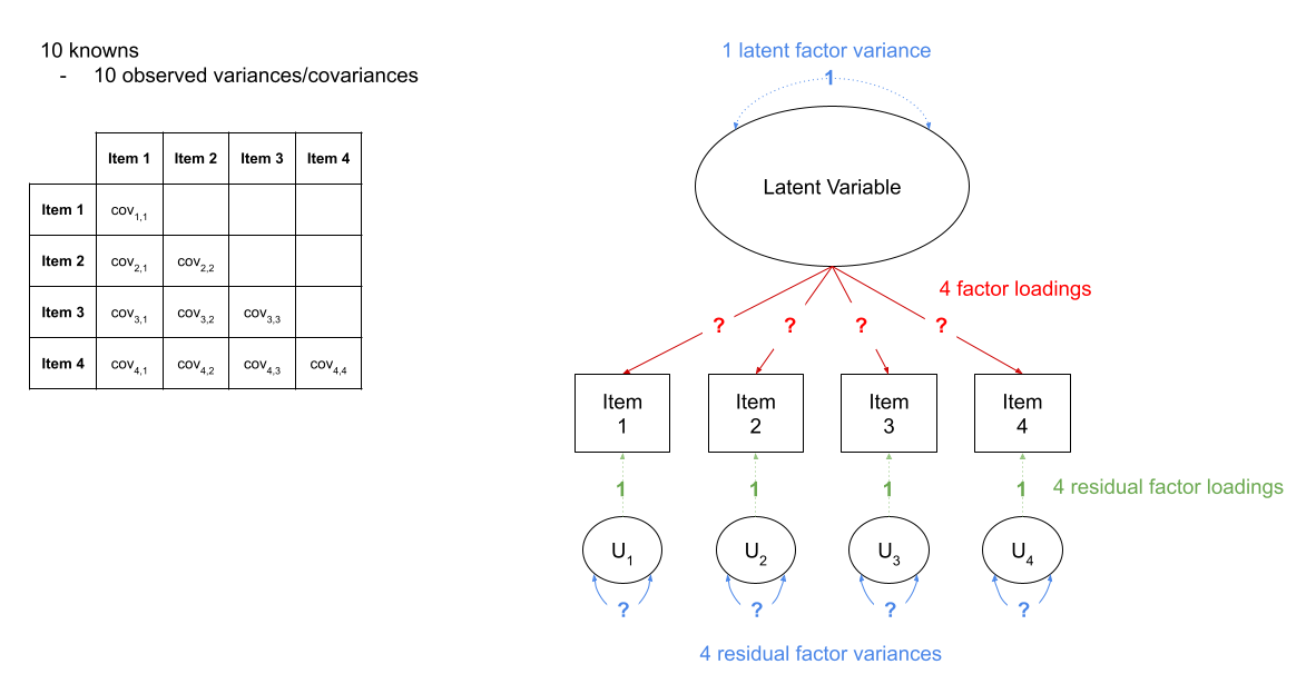
Latent Variable Scaling

in Figure 2, we can see a the model of a latent factor loading on to 4 items. The number of paths to be estimated here is greater than the number of known covariances. However, we can get around this by fixing certain parameters to be specific values. In Figure 3, the latent factor variance is set at 1, and the residual factor loadings are also set to 1.
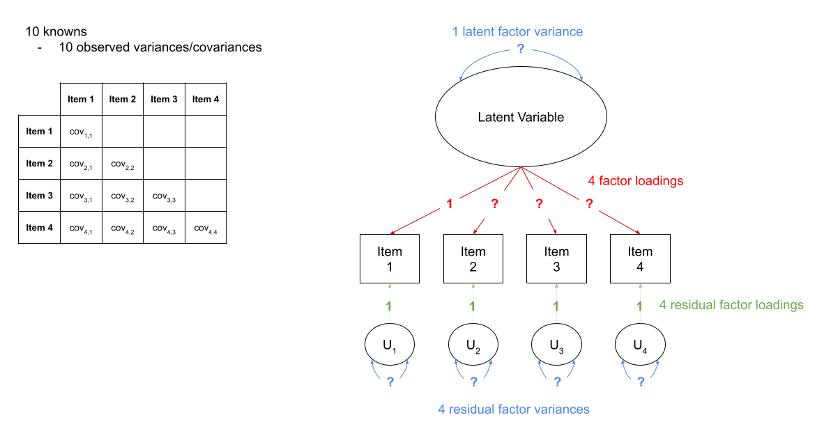
This has the additional benefit of making our latent factor have some defining features. Because we don’t actually measure the latent variable (it is a hypothetical construct), it doesn’t really have any intrinsic ‘scale’. When we fix the variance to be 1, we are providing some property (its variance) we create a reference from which the other paths to/from the variable are in relation to. A common alternative is to fix the factor loading of the first item to be 1 (see Figure 4).

Figure 2: A four item factor structure. There are 10 knowns, but 13 parameters

Figure 3: A four item factor structure. By fixing 5 of these parameters to be equal to 1, we gain back degrees of freedom and make our model identifiable

Figure 4: A four item factor structure. The ‘marker method’ fixes the first factor loading to be 1, leaving the factor variance free to be estimated.

Fit the model again, (assign it a new name so we can compare), but this time use:

cfa(model_syntax, data = ..., std.lv = TRUE)

Do the fit measures such as TLI, CFI, RMSEA, SRMR etc., change at all? Do the loadings change at all? Can you see a link between these loadings and those from the previously fitted model?

Here’s our original model:

cpmod.est <- cfa(cpmod, data = cp2)

Here’s our model with std.lv=TRUE:

cpmod.est2 <- cfa(cpmod, data = cp2, std.lv=TRUE)

The fit is identical! This is much like how lm(y~x) and lm(scale(y)~scale(x)) are one and the same model - the difference only comes in the estimates being transformed to be in different scales.

fitmeasures(cpmod.est)[c("srmr","rmsea","tli","cfi")]

      srmr      rmsea        tli        cfi 
0.03454489 0.03945991 0.98494172 0.98862263 

fitmeasures(cpmod.est2)[c("srmr","rmsea","tli","cfi")]

      srmr      rmsea        tli        cfi 
0.03454489 0.03945991 0.98494172 0.98862263 

The loadings from the model with std.lv=TRUE are all <1.

summary(cpmod.est2)

...

Latent Variables:
                   Estimate  Std.Err  z-value  P(>|z|)
  nonagg =~                                           
    item1             0.673    0.039   17.402    0.000
    item2             0.819    0.039   21.024    0.000
    item3             0.681    0.038   17.816    0.000
    item4             0.771    0.041   18.876    0.000
    item5             0.915    0.036   25.425    0.000
  agg =~                                              
    item6             0.618    0.037   16.793    0.000
    item7             0.877    0.033   26.319    0.000
    item8             0.887    0.032   28.087    0.000
    item9             0.675    0.038   17.875    0.000
    item10            0.587    0.037   15.872    0.000

...

Taking just the first factor, note that the first loading is 0.673. Relative to this loading, the other loadings of 0.819, 0.681, 0.771, 0.915, are all bigger. How much bigger?
If we divide each one by that first loading, we get their size relative to that loading - these are the same as our unstandardised loadings!

\(\frac{0.819}{0.673}=1.217\)
\(\frac{0.681}{0.673}=1.012\)
\(\frac{0.771}{0.673}=1.146\)
\(\frac{0.915}{0.673}=1.360\)

Note also that we now have fixed values for the variances of the latent factors, which previously were being estimated for us.

In the second model, with std.lv=TRUE:

...
Variances:
                   Estimate  Std.Err  z-value  P(>|z|)
    nonagg            1.000                           
    agg               1.000                           
...

And in the first:

...
Variances:
                   Estimate  Std.Err  z-value  P(>|z|)
    nonagg            0.453    0.052    8.701    0.000
    agg               0.381    0.045    8.396    0.000
...

Question Optional 5

We don’t actually even have to re-fit the model in order to get out standardised estimates.

Try doing:

mod.est <- cfa(model_syntax, data = ...)
summary(mod.est, std=TRUE)

You’ll get some extra columns - can you figure out what they are?

Back to our original model fit:

cpmod.est <- cfa(cpmod, data = cp2)

We get out an extra couple of columns here. One of which we have already seen - the Std.lv column contains the same numbers from the previous question. The numbers in the Std.all column are similar, but not quite the same.

summary(mod.est, std=TRUE)

...

Latent Variables:
                   Estimate  Std.Err  z-value  P(>|z|)   Std.lv  Std.all
  nonagg =~                                                             
    item1             1.000                               0.673    0.664
    item2             1.217    0.076   15.965    0.000    0.819    0.765
    item3             1.012    0.070   14.424    0.000    0.681    0.676
    item4             1.146    0.077   14.967    0.000    0.771    0.706
    item5             1.360    0.078   17.412    0.000    0.915    0.872
  agg =~                                                                
    item6             1.000                               0.618    0.636
    item7             1.419    0.082   17.331    0.000    0.877    0.878
    item8             1.437    0.081   17.662    0.000    0.887    0.915
    item9             1.093    0.077   14.125    0.000    0.675    0.668
    item10            0.950    0.073   13.073    0.000    0.587    0.608

...

The Std.lv column represents when the latent variables are scaled to have a variance of 1, but the measured variables variances are not.
The Std.all column represents when both latent variables and measured variable are scaled to have variances of 1.

This means that if we first standardised all our observed variables manually, and then fitted our model to that data, then the Std.lv and Std.all columns would be identical.

Question 6

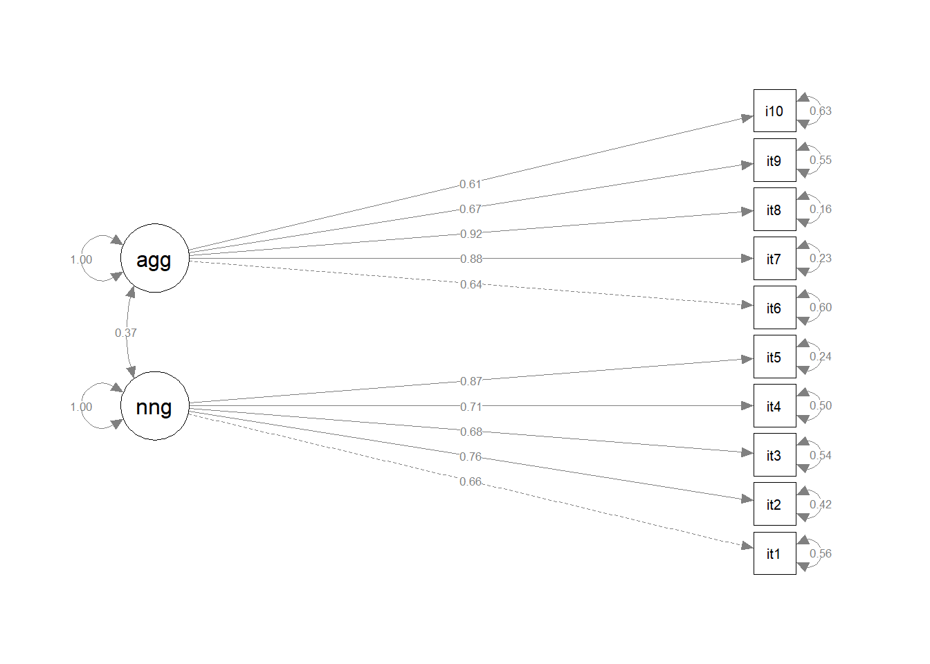
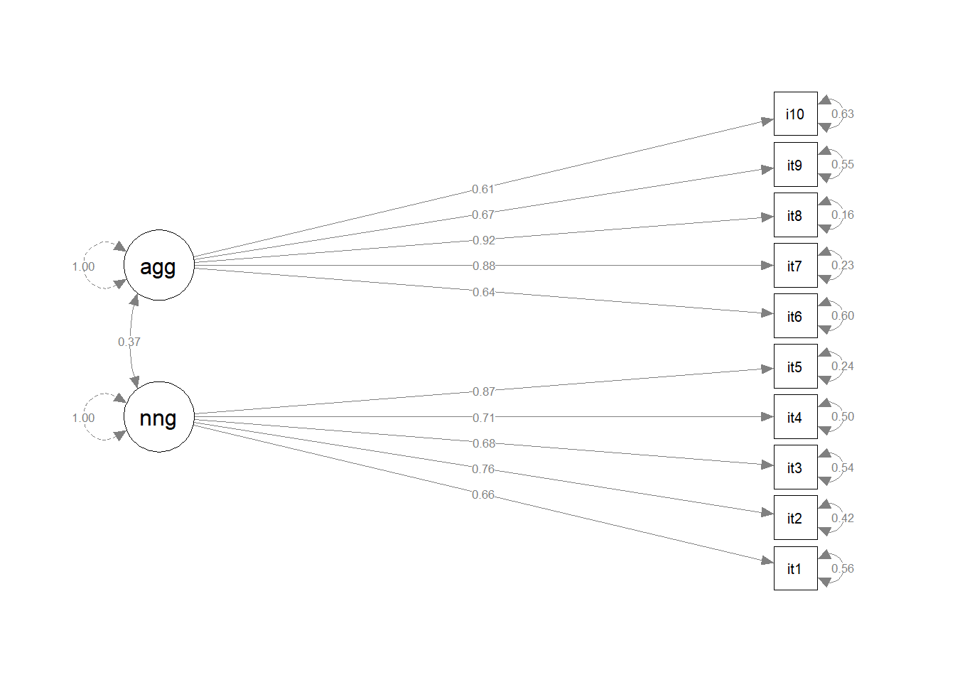
Make a diagram of your model, using the standardised factor loadings as labels.

The semPlot package

For more complex models with latent variables, we will almost always have to make diagrams manually, either in generic presentation software such as powerpoint or google slides, or in specific software such as semdiag.

R has a couple of packages which work well enough for some of the more common model structures such as CFA.

The semPaths() function from semPlot package can take a fitted lavaan model and create a nice diagram.

library(semPlot)
semPaths(myfittedmodel, 
        what = ?, # line thickness & color by... 
        whatLabels = ?, # label lines as... 
        rotation = ? # rotations, +1 = 90degrees
        )

optional: handy functionality!

Occasionally we might want to draw models before we even get the data. lavaan has some useful functionality where you can give it a model formula and ask it to “lavaanify” it into a model object that just hasn’t yet been fitted to anything.

For instance, by setting up a pretend model and “lavaanify-ing” it, we can then make a diagram!

pretend_model <- "
biscuits =~ digestive + oreo + custard_cream + bourbon + crackers
crisps =~ salt_vinegar + cheese_onion + prawn_cocktail + crackers
"
lavaanify(pretend_model) |>
  semPaths()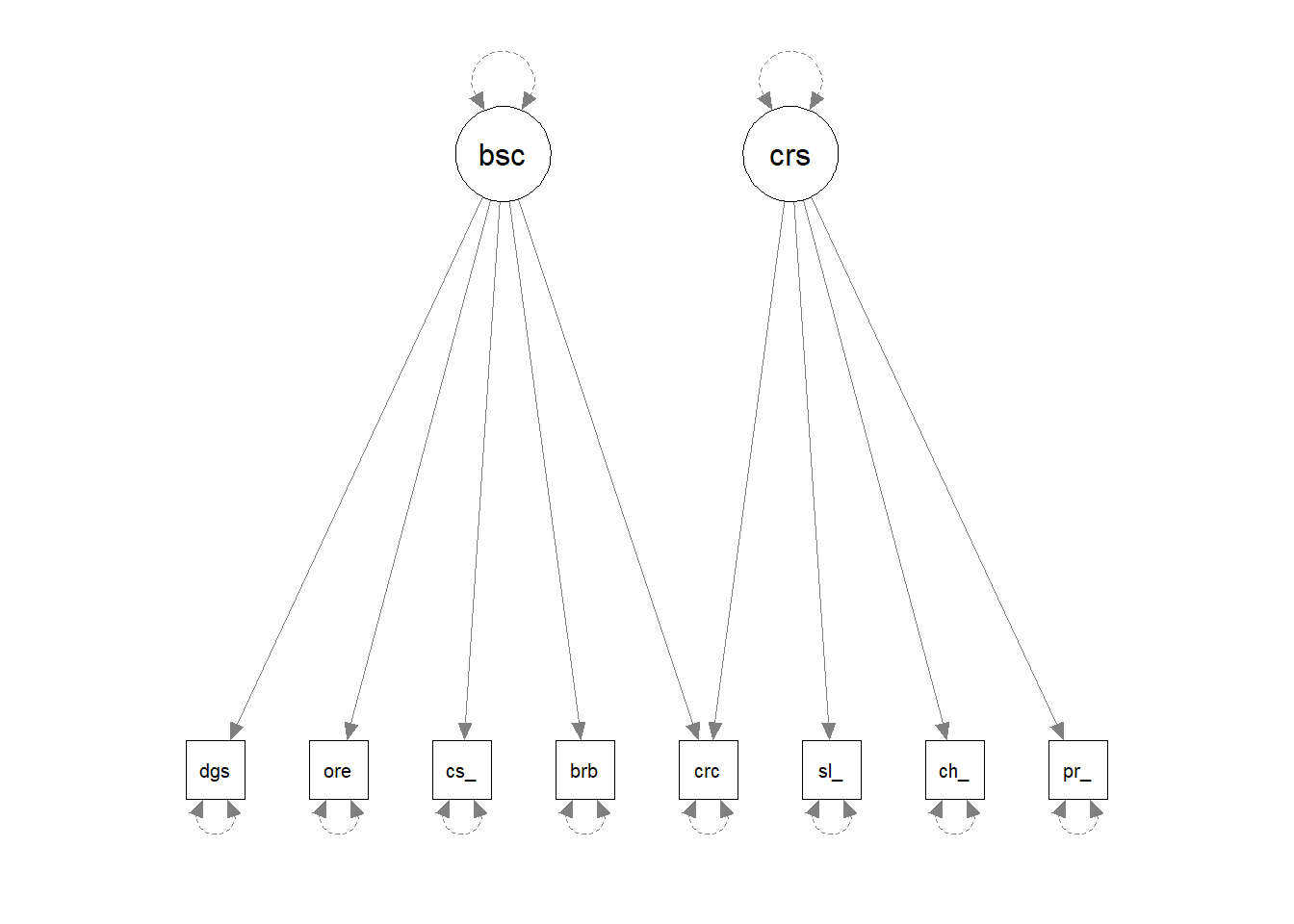

You can rotate this however you like. Convention is typically to have it downwards but I like it left to right (not sure why!)

library(semPlot)
semPaths(cpmod.est, 
        whatLabels = "std", 
        rotation = 2)

The lines from agg =~ item6 and nonagg =~ item1 are dotted to indicate that the model was initially fitted with the loading fixed to 1. Because we’re showing standardised loadings, we could just use the model when fitted with std.lv=TRUE just to stop these dotted lines from appearing:

library(semPlot)
semPaths(cpmod.est2, 
        whatLabels = "std", 
        rotation = 2)

Question 7

Make a bullet point list of everything you have done so far, and the resulting conclusions.
Then, if you feel like it, turn the bulleted list into written paragraphs, and you’ll have a write-up of your analyses!

A two-factor model was tested. Items 1-5 loaded on a ‘non-aggressive conduct problems’ factor and items 6-10 loaded on an ‘aggression’ factor and these factors were allowed to correlate. Scaling and identification were achieved by fixing the loading of item 1 on the non-aggressive conduct problems factor and item 6 on the aggression factor to 1. The model was estimated using maximum likelihood estimation. The model fit well with CFI=.99, TLI=0.99, RMSEA=.04, and SRMR=.04 (Hu & Bentler, 1999). All loadings were statistically significant and >|.3| on the standardised scale. Overall, therefore, a two-factor oblique model was supported for the conduct problems items. The correlation between the factors was \(r=.38\,\, (p<.001)\).

parameter	est	std.est	se	z	pvalue
nonagg=~item1	1.000	0.664	0.000
nonagg=~item2	1.217	0.765	0.076	15.965	< 0.001
nonagg=~item3	1.012	0.676	0.070	14.424	< 0.001
nonagg=~item4	1.146	0.706	0.077	14.967	< 0.001
nonagg=~item5	1.360	0.872	0.078	17.412	< 0.001
agg=~item6	1.000	0.636	0.000
agg=~item7	1.419	0.878	0.082	17.331	< 0.001
agg=~item8	1.437	0.915	0.081	17.662	< 0.001
agg=~item9	1.093	0.668	0.077	14.125	< 0.001
agg=~item10	0.950	0.608	0.073	13.073	< 0.001
nonagg~~agg	0.156	0.375	0.023	6.856	< 0.001
item1~~item1	0.574	0.559	0.037	15.398	< 0.001
item2~~item2	0.477	0.416	0.035	13.778	< 0.001
item3~~item3	0.551	0.543	0.036	15.262	< 0.001
item4~~item4	0.597	0.501	0.040	14.867	< 0.001
item5~~item5	0.264	0.239	0.028	9.537	< 0.001
item6~~item6	0.561	0.595	0.035	16.193	< 0.001
item7~~item7	0.228	0.229	0.021	10.767	< 0.001
item8~~item8	0.153	0.162	0.019	8.122	< 0.001
item9~~item9	0.566	0.554	0.035	15.978	< 0.001
item10~~item10	0.587	0.630	0.036	16.351	< 0.001
nonagg~~nonagg	0.453	1.000	0.052	8.701	< 0.001
agg~~agg	0.381	1.000	0.045	8.396	< 0.001

“DOOM” Scrolling

Dataset: doom.csv

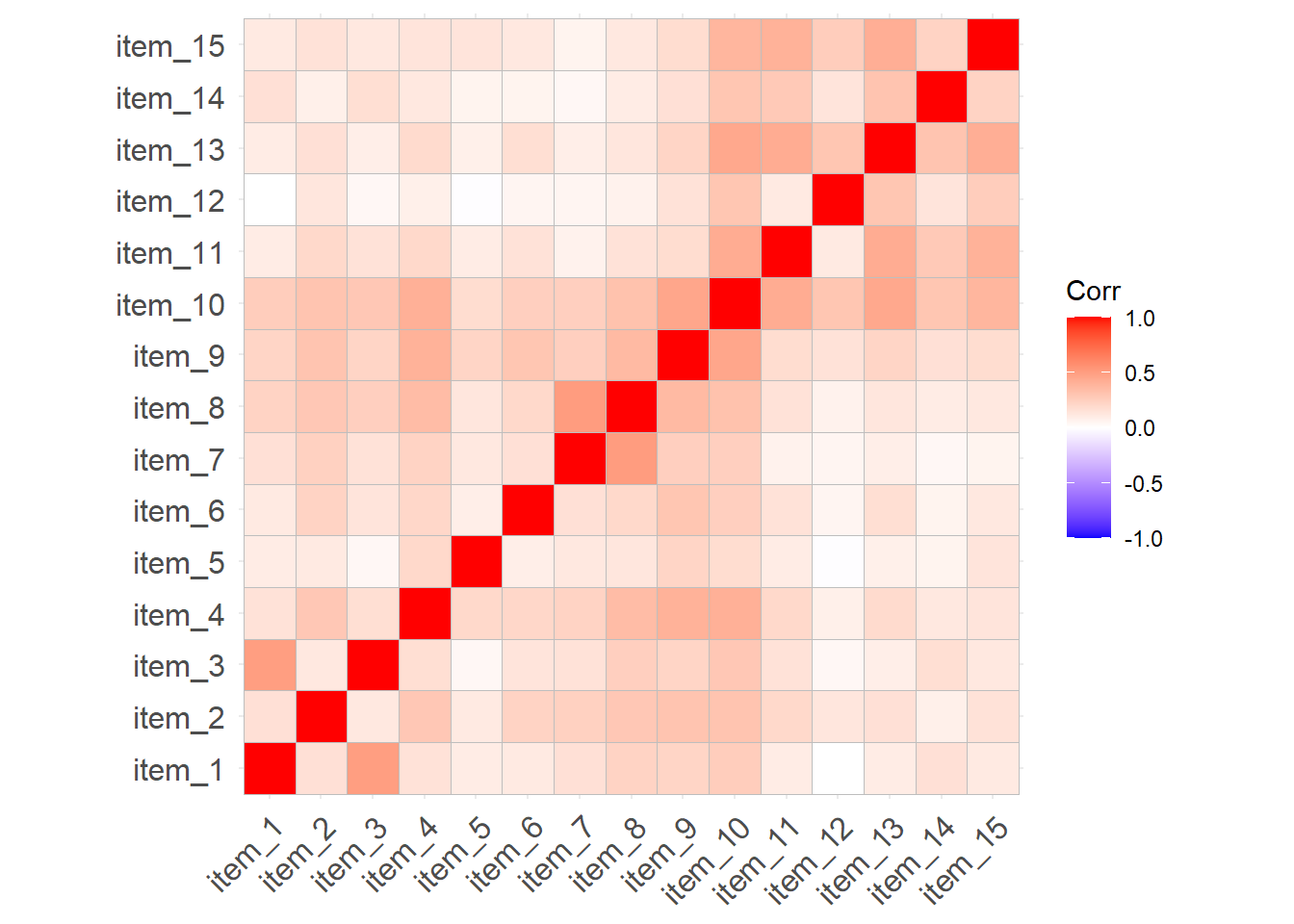
The “Domains of Online Obsession Measure” (DOOM) is a fictitious scale that aims to assess the sub types of addictions to online content. It was developed to measure 2 separate domains of online obsession: items 1 to 9 are representative of the “emotional” relationships people have with their internet usage (i.e. how it makes them feel), and items 10 to 15 reflect “practical” relationship (i.e., how it connects or interferes with their day-to-day life). Each item is measured on a 7-point likert scale from “strongly disagree” to “strongly agree”.

We administered this scale to 476 participants in order to assess the validity of the 2 domain structure of the online obsession measure that we obtained during scale development.

The data are available at https://uoepsy.github.io/data/doom.csv, and the table below shows the individual item wordings.

variable	question
item_1	i just can't stop watching videos of animals
item_2	i spend hours scrolling through tutorials but never actually attempt any projects.
item_3	cats are my main source of entertainment.
item_4	life without the internet would be boring, empty, and joyless
item_5	i try to hide how long i’ve been online
item_6	i avoid thinking about things by scrolling on the internet
item_7	everything i see online is either sad or terrifying
item_8	all the negative stuff online makes me feel better about my own life
item_9	i feel better the more 'likes' i receive
item_10	most of my time online is spent communicating with others
item_11	my work suffers because of the amount of time i spend online
item_12	i spend a lot of time online for work
item_13	i check my emails very regularly
item_14	others in my life complain about the amount of time i spend online
item_15	i neglect household chores to spend more time online

Question 8

Assess whether the 2 domain model of online obsession provides a good fit to the validation sample of 476 participants.

From the visual of the correlation matrix, you can see the vague outline of two groups of items correlations. Note there’s a little overlap..

doom <- read_csv("https://uoepsy.github.io/data/doom.csv")
ggcorrplot(cor(doom))

first we write our model:

moddoom <- "
# emotional domain
emot =~ item_1 + item_2 + item_3 + item_4 + item_5 + item_6 + item_7 + item_8 + item_9
# practical domain
pract =~ item_10 + item_11 + item_13 + item_14 + item_15
# correlated domains (will be estimated by default)
emot ~~ pract
"

Then we fit it to the data:

moddoom.est <- cfa(moddoom, data = doom)

Then we inspect that fitted model object.
I’m just going to extract the fit indices here first.

fitmeasures(moddoom.est)[c("rmsea","srmr","cfi","tli")]

     rmsea       srmr        cfi        tli 
0.07331272 0.06227484 0.84791972 0.81790388 

Uh-oh.. they don’t look great.

Question 9

Are there any areas of local misfit (certain parameters that are not in the model (and are therefore fixed to zero) but that could improve model fit if they were estimated?).

modification indices

When a factor structure does not fit well, we can either start over and go back to doing EFA, deciding on an appropriate factor structure, on whether we should drop certain items, etc. The downside of this is that we essentially result in another version of the scale, and before we know it, we have 10 versions of the same measure floating around, in a perpetual state of scale-development. Alternatively, we can see if it is possible to minimally adjust our model based on areas of local misfit in order to see if our global fit improves. Note that this would still be in a sense exploratory, and we should be very clear when writing up about the process that we undertook. We should also avoid just shoving any parameter in that might make it fit better - we should let common sense and theoretical knowledge support any adjustments we make.

The modindices() function takes a fitted model object from lavaan and provides a table of all the possible additional parameters we could estimate.

The output is a table, which we can ask to be sorted according to the mi column using sort = TRUE.

modindices(myfittedmodel, sort = TRUE)

      lhs op    rhs     mi    epc sepc.lv sepc.all sepc.nox
72  item6 ~~ item10 10.747  0.082   0.082    0.144    0.144
25 fact1  =~  item7  8.106  0.119   0.080    0.080    0.080
65  item5 ~~  item7  6.720  0.039   0.039    0.160    0.160
71  item6 ~~  item9  6.675 -0.065  -0.065   -0.115   -0.115
.   ...   .   ...    ...    ...     ...      ...      ...

The columns show:

lhs,op,rhs	mi	epc	sepc.lv, sepc.all,sepc.nox
these three columns show the specific parameter, in lavaan syntax. So fact1 =~ item7 is for the possible inclusion of item7 being loaded on to the latent variable fact1. item6 ~~ item10 is for the inclusion of a covariance between item6 and item10, and so on.	“modification index” = the change in the model \(\chi^2\) value were we to include this parameter in the model	“expected parameter change” = the estimated value that the parameter would take were it included in the model	these provide the epc values but scaled to when a) the latent variables are standardised, b) all variables are standardised, and c) all except exogenous observed variables are standardised (not relevant for CFA)

Often, the sepc.allis a useful column to look at, because it shows the proposed parameter estimate in a standardised metric. i.e. if the op is ~~, then the sepc.all value is a correlation, and so we can consider anything <.2/.3ish to be quite small. If op is =~, then the sepc.all value is a standardised factor loading, so values >.3 or >.4 are worth thinking about, and so on.

I’m printing out just the head(), so that I can look at the few parameters with the greatest modification indices.
The top three parameters jump out immediately to me.
item_1 and item_3 have a suggested correlation of c0.5, as do item_7 and item_8. In addition, it’s suggested that including a loading (estimated to be about 0.6) from item_10 to the emot factor would improve the model fit.

modindices(moddoom.est, sort=TRUE) |>
  head()

        lhs op     rhs     mi    epc sepc.lv sepc.all sepc.nox
47   item_1 ~~  item_3 88.700  0.560   0.560    0.459    0.459
32     emot =~ item_10 74.374  1.690   0.817    0.640    0.640
109  item_7 ~~  item_8 61.930  0.370   0.370    0.432    0.432
34     emot =~ item_13 14.824 -0.655  -0.317   -0.275   -0.275
122  item_9 ~~ item_10 12.634  0.145   0.145    0.217    0.217
135 item_13 ~~ item_15  8.956  0.178   0.178    0.171    0.171

Question 10

Beware: there’s a slightly blurred line here that we’re about to step over, and move from confirmatory back to ‘exploratory’.

Look carefully at the item wordings,do any of the suggested modifications make theoretical sense? Add them to the model and re-fit it. Does this new model fit well?

model modifications are exploratory!!

It’s likely you will have to make a couple of modifications in order to obtain a model that fits well to this data.

BUT… we could simply keep adding suggested parameters to our model and we will eventually end up with a perfectly fitting model.

It’s very important to think critically here about why such modifications may be necessary.

• The initial model may have failed to capture the complexity of the underlying relationships among variables. For instance, suggested residual covariances, representing unexplained covariation among observed variables, may indicate misspecification in the initial model.
• The structure of the construct is genuinely different in your population from the initial one in which the scale is developed (this could be a research question in and of itself - i.e. does the structure of “anxiety” differ as people age, or differ between cultures?)

Modifications to a CFA model should be made judiciously, with careful consideration of theory as well as quantitative metrics. The goal is to develop a model that accurately represents the underlying structure of the data while maintaining theoretical coherence and generalizability.

In this case, the likely reason for the poor fit of the “DOOM” scale, is that the person who made the items (ahem, me) doesn’t really know anything about the construct they are talking about, and didn’t put much care into constructing the items!

There are three main proposed adjustments from our initial model:

1. item_1 ~~ item_3. These questions are both about animals. It would make sense that these are related over and above the underlying “emotional internet usage” factor.

2. item_7 ~~ item_8. These are both about viewing negative content online, so it makes sense here that they would be related beyond the ‘emotional’ factor.

3. emot =~ item_10. This item is about communicating with others. It currently loads highly on the pract factor too. It maybe makes sense here that “communicating with others” will capture both a practical element of internet useage and an emotional one.

Putting them all in at once could be a mistake - if we added in emot =~ item_10, then we change slightly the underlying construct of the emot factor, meaning it might make other suggested modifications (item_7 ~~ item_8) less important. It’s a bit like Whac-A-Mole - you make one modification and then a whole new area of misfits appears!

Let’s adjust our model:

moddoom2 <- "
# emotional domain
emot =~ item_1 + item_2 + item_3 + item_4 + item_5 + item_6 + item_7 + item_8 + item_9 + item_10
# practical domain
pract =~ item_10 + item_11 + item_13 + item_14 + item_15
# correlated domains (will be estimated by default)
emot ~~ pract
"

Then fit it to the data:

moddoom2.est <- cfa(moddoom2, data = doom)

fitmeasures(moddoom2.est)[c("rmsea","srmr","cfi","tli")]

     rmsea       srmr        cfi        tli 
0.06013775 0.05147585 0.89901514 0.87747171 

The fit is still not great, and the same suggested correlations are present in modification indices:

modindices(moddoom2.est, sort=TRUE) |>
  head()

       lhs op     rhs     mi    epc sepc.lv sepc.all sepc.nox
47  item_1 ~~  item_3 87.679  0.553   0.553    0.455    0.455
109 item_7 ~~  item_8 61.827  0.365   0.365    0.421    0.421
43   pract =~  item_7  7.117 -0.300  -0.178   -0.159   -0.159
48  item_1 ~~  item_4  6.264 -0.139  -0.139   -0.128   -0.128
117 item_8 ~~ item_10  6.072 -0.110  -0.110   -0.151   -0.151
44   pract =~  item_8  5.065 -0.244  -0.145   -0.130   -0.130

Let’s go ahead and put the covariance between item_1 and item_3 in. I personally went for this first because they seem more similar to me than item_7 and item_8 do.

moddoom3 <- "
# emotional domain
emot =~ item_1 + item_2 + item_3 + item_4 + item_5 + item_6 + item_7 + item_8 + item_9 + item_10
# practical domain
pract =~ item_10 + item_11 + item_13 + item_14 + item_15
# correlated domains (will be estimated by default)
emot ~~ pract
item_1 ~~ item_3
"

moddoom3.est <- cfa(moddoom3, data = doom)

fitmeasures(moddoom3.est)[c("rmsea","srmr","cfi","tli")]

     rmsea       srmr        cfi        tli 
0.03282045 0.03830848 0.97032291 0.96350520 

Whoop! It fits well! It may well be that if we inspect modification indices again, we still see that item_1 ~~ item_3 would improve our model fit. The thing to remember however, is that we could simply keep adding parameters until we run out of degrees of freedom, and our model would “fit better”. But such a model would not be useful. It would not generalise well, becaue it runs the risk of being overfitted to the nuances of this specific sample.

Optional Extra Exercises for the Enthusiastic

Dataset: radakovic_das.csv

Apathy is lack of motivation towards goal-directed behaviours. It is pervasive in a majority of psychiatric and neurological diseases, and impacts everyday life. Traditionally, apathy has been measured as a one-dimensional construct but is in fact composed of different types of demotivation.

Dimensional Apathy Scale (DAS) The Dimensional Apathy Scale (DAS) is a multidimensional assessment for demotivation, in which 3 subtypes of apathy are assessed:

• Executive: lack of motivation for planning, attention or organisation
• Emotional: lack of emotional motivation (indifference, affective or emotional neutrality, flatness or blunting)
• Initiation: lack of motivation for self-generation of thoughts and/or actions

The DAS measures these subtypes of apathy and allows for quick and easy assessment, through self-assessment, observations by informants/carers or administration by researchers or healthcare professionals.

You can find data for the DAS when administered to 250 healthy adults at https://uoepsy.github.io/data/radakovic_das.csv, and information on the items is below.

DAS Dictionary

All items are measured on a 6-point Likert scale of Always (0), Almost Always (1), Often (2), Occasionally (3), Hardly Ever (4), and Never (5). Certain items (indicated in the table below with a - direction) are reverse scored to ensure that higher scores indicate greater levels of apathy.

item	direction	dimension	question
1	+	Executive	I need a bit of encouragement to get things started
2	-	Initiation	I contact my friends
3	-	Emotional	I express my emotions
4	-	Initiation	I think of new things to do during the day
5	-	Emotional	I am concerned about how my family feel
6	+	Executive	I find myself staring in to space
7	-	Emotional	Before I do something I think about how others would feel about it
8	-	Initiation	I plan my days activities in advance
9	-	Emotional	When I receive bad news I feel bad about it
10	-	Executive	I am unable to focus on a task until it is finished
11	+	Executive	I lack motivation
12	+	Emotional	I struggle to empathise with other people
13	-	Initiation	I set goals for myself
14	-	Initiation	I try new things
15	+	Emotional	I am unconcerned about how others feel about my behaviour
16	-	Initiation	I act on things I have thought about during the day
17	+	Executive	When doing a demanding task, I have difficulty working out what I have to do
18	-	Initiation	I keep myself busy
19	+	Executive	I get easily confused when doing several things at once
20	-	Emotional	I become emotional easily when watching something happy or sad on TV
21	+	Executive	I find it difficult to keep my mind on things
22	-	Initiation	I am spontaneous
23	+	Executive	I am easily distracted
24	+	Emotional	I feel indifferent to what is going on around me

Question 11

Read in the data. It will need a little bit of tidying before we can get to fitting a CFA.
If you haven’t already, check out the page on Data Wrangling for Surveys & Questionnaires.

First let’s just read in the dataset:

rdas <- read_csv("https://uoepsy.github.io/data/radakovic_das.csv")
head(rdas)

# A tibble: 6 × 24
  I need a bit of encouragement …¹ `I contact my friends` I express my emotion…²
  <chr>                            <chr>                  <chr>                 
1 Often                            Almost Always          Almost Always         
2 Almost Always                    Hardly Ever            Occasionally          
3 Often                            Occasionally           Occasionally          
4 Hardly Ever                      Occasionally           Almost Always         
5 Occasionally                     Hardly Ever            Occasionally          
6 Occasionally                     Occasionally           Almost Always         
# ℹ abbreviated names: ¹​`I need a bit of encouragement to get things started`,
#   ²​`I express my emotions`
# ℹ 21 more variables: `I think of new things to do during the day` <chr>,
#   `I am concerned about how my family feel` <chr>,
#   `I find myself staring in to space` <chr>,
#   `Before I do something I think about how others would feel about it` <chr>,
#   `I plan my days activities in advance` <chr>, …

The names we’re getting are useful in that they show the items, but they’re horrible to have to use in R, so we will ideally replace them with easy to use names. Note also that the data is being read in as the actual response option - e.g., “Almost Always” - and we want to treat these as a numeric scale. So those will have to change too.

I like to make a “data dictionary” whenever I get data like this. While I want to rename the variables to make it easier for me to use, I also want to keep track of what the questions were.
Here I make a “tibble” (the function data.frame() would work too, tibble is just tidyverse version). I indicate what I am going to rename things as (“q1”,“q2”, …, “q24”), and then I have the current names of the variables

rdas_dict <- tibble(
  variable = paste0("q",1:24),
  item = names(rdas)
)

Doing this is really useful because I can’t keep track in my head of what “q5” was.
If I want to know, then I can just do:

rdas_dict[5,]

# A tibble: 1 × 2
  variable item                                   
  <chr>    <chr>                                  
1 q5       I am concerned about how my family feel

Now let’s actually change the names in our data to what we said we would:

names(rdas) <- paste0("q", 1:24)

Okay, so we have all our data in words, not numbers. Views on how to treat Likert data are mixed, but it’s very common to treat it as continuous in Psychology.

Let’s check the response values we have. Just in question 1 for now:

unique(rdas$q1)

[1] "Often"         "Almost Always" "Hardly Ever"   "Occasionally" 
[5] "Always"        NA              "Never"        

A little trick that we can use to find the unique values in an entire dataset is to quickly convert the dataframe into one big long vector. Technically, a dataframe is a “list of vectors”, and the function unlist() will remove this structure.
So we can find all the unique values in all the questions with:

unique(unlist(rdas))

[1] "Often"         "Almost Always" "Hardly Ever"   "Occasionally" 
[5] "Always"        NA              "Never"         "[NO ENTRY]"   

Perfect. So we know we have uniformity of spelling. It happens less often these days as questionnaire software is improving, but you might occasionally encounter typos in some of the questions, or things with and without capital letters (R is a bit thick, and doesn’t recognise that “Often” and “often” are the same thing).
Note that we have the 6 responses that we would expect given the description of the scale, but we also have some NA values, and some [NO ENTRY] values. Not sure how those got there.
We want to turn each “Always” in to 0, each “Almost Always” in to 1, “Often” in to 2, and so on. If we simply leave out the “[NO ENTRY]”, then this will be turned into a missing value NA, which is handy.

rdas <- rdas |> 
  mutate(across(q1:q24, ~case_match(.,
    "Always" ~ 0,
    "Almost Always" ~ 1,
    "Often" ~ 2,
    "Occasionally" ~ 3,
    "Hardly Ever" ~ 4,
    "Never" ~ 5
  )))
head(rdas)

# A tibble: 6 × 24
     q1    q2    q3    q4    q5    q6    q7    q8    q9   q10   q11   q12   q13
  <dbl> <dbl> <dbl> <dbl> <dbl> <dbl> <dbl> <dbl> <dbl> <dbl> <dbl> <dbl> <dbl>
1     2     1     1     4     1     3     1     4     2     2     3     2     3
2     1     4     3     4    NA     0    NA     2    NA     2     1     2     3
3     2     3     3     4     3     3     2     2     4     1     3     2     3
4     4     3     1     3     1    NA     2     2    NA     2     3     4     2
5     3     4     3     5     2     2     2     3     3     2     2     2     1
6     3     3     1     0     1     2     1     1     0     2     1     4     3
# ℹ 11 more variables: q14 <dbl>, q15 <dbl>, q16 <dbl>, q17 <dbl>, q18 <dbl>,
#   q19 <dbl>, q20 <dbl>, q21 <dbl>, q22 <dbl>, q23 <dbl>, q24 <dbl>

We haven’t learned about more sophisticated methods of handling missing data, so for now we will just remove any rows in which there is missingness - i.e., we’ll do “listwise deletion”:

compl_rdas <- na.omit(rdas)

Question 12

How well does the 3-dimensional model of apathy fit to this dataset?

Hints

You’ll have to use the data dictionary to figure out which items are associated with with dimensions.

Here is the model structure, according to the list of items in the dictionary.
I’m calling my factors “Em”, “Ex”, and “BCI” for “emotional”, “executive” and “behavioural/cognitive initiation” respectively. The factor correlations will be estimated by default, but I like to write things explicitly.

dasmod = "
Em =~ q1 + q6 + q10 + q11 + q17 + q19 + q23
Ex =~ q3 + q5 + q7 + q9 + q12 + q15 + q20 + q24
BCI =~ q2 + q4 + q8 + q13 + q14 + q16 + q18 + q22
Em ~~ Ex
Em ~~ BCI
Ex ~~ BCI
"

Let’s fit the model!

dasmod.est = cfa(dasmod, compl_rdas)

And examine the global fit:

fitmeasures(dasmod.est)[c("srmr","rmsea","tli","cfi")]

      srmr      rmsea        tli        cfi 
0.05484788 0.02614997 0.95698828 0.96140846 

All looks pretty good! Cut-offs for SRMR tend to vary, with some using <0.08, or <0.09, and some being stricter with <0.05. Remember, these criteria are somewhat arbitrary.

Modification indices suggest a whole bunch of items that could have some associations beyond that modelled in the factors, but these are all weak correlations at around 0.2.

modindices(dasmod.est, sort=TRUE) |> head()

    lhs op rhs     mi    epc sepc.lv sepc.all sepc.nox
126  q6 ~~  q3 15.790 -0.221  -0.221   -0.284   -0.284
108  q1 ~~  q9 11.413  0.169   0.169    0.264    0.264
206 q19 ~~ q20 10.884 -0.167  -0.167   -0.257   -0.257
331  q4 ~~  q8  7.552  0.201   0.201    0.208    0.208
99   q1 ~~  q6  7.310  0.150   0.150    0.224    0.224
101  q1 ~~ q11  6.183 -0.149  -0.149   -0.236   -0.236

These are the top 3 being suggested. I can’t see any obvious link between any of these that would make me think they are related beyond their measuring of ‘apathy’.

rdas_dict[c(3,6),]

# A tibble: 2 × 2
  variable item                             
  <chr>    <chr>                            
1 q3       I express my emotions            
2 q6       I find myself staring in to space

rdas_dict[c(1,9),]

# A tibble: 2 × 2
  variable item                                               
  <chr>    <chr>                                              
1 q1       I need a bit of encouragement to get things started
2 q9       When I receive bad news I feel bad about it        

rdas_dict[c(19,20),]

# A tibble: 2 × 2
  variable item                                                                
  <chr>    <chr>                                                               
1 q19      I get easily confused when doing several things at once             
2 q20      I become emotional easily when watching something happy or sad on TV

Question 13

Much like for EFA, we can estimate individuals’ scores on the latent factors. In lavaan, the function lavPredict() will get us some estimates.

However, for a clinician administering the DAS to a patient, this option is not available. Instead, it is common that scores on the individual items associated with a given factor are used to create a sum score or a mean score which can be used in a practical setting (e.g., scores above a given threshold might indicate cause for concern).

Calculate sum scores for each of the dimensions of apathy.

Hints

You’ll need to reverse some items first! See Data Wrangling for Surveys #reverse-coding.

According to the table of items, the ones which need to be reverse scored are:

reversed <- c(2,3,4,5,7,8,9,10,13,14,16,18,20,22)

For these items, we want 5s to become 0s, 4s become 1s, and so on..

compl_rdas[, reversed] <- apply(
  compl_rdas[, reversed], MARGIN = 2, function(x) 5-x)

Note: The above code works nicely because our dataset is currently ordered such that the first column is item 1, 2nd column is item 2, and so on. This means we can use numbers to index the appropriate variables, rather than names. It would need adjusting if, for instance, our first column contained “participant ID”, and our items only began later.

Here are the sets of items associated with each dimension:

Exitems <- c(1,6,10,11,17,19,21,23)
Emitems <- c(3,5,7,9,12,15,20,24)
BCIitems <- c(2,4,8,13,14,16,18,22)

Again, because the item numbers correspond to the column positions in our data, we can just do rowSums indexing on those column numbers to get our scores:

compl_rdas$ExSCORE <- rowSums(compl_rdas[,Exitems])
compl_rdas$EmSCORE <- rowSums(compl_rdas[,Emitems])
compl_rdas$BCIScore <- rowSums(compl_rdas[,BCIitems])

optional: what is a sum score but a constrained factor model?

Computing sum scores can feel like a ‘model free’ calculation, but actually it does pre-suppose a factor structure, and a much more constrained one than those we have been estimating. For a full explanation of this, see “Thinking twice about sum scores”, McNeish & Wolf 2020.

Footnotes

1. or in logistic regression, “what is the likelihood of observing the outcome \(y\) given our model parameters?”