Week 5 Exercises: Assumptions, Diagnostics, Writing up

Video game aggression and the dark triad

Dataset: NGV.csv

These data are from an experiment designed to investigate how the realism of video games is associated with more/less unnecessarily aggressive gameplay, and whether this differs depending upon a) the playing mode (playing on a screen vs VR headset), and b) individual differences in the ‘dark triad’ personality traits.

The experiment involved playing 10 levels of a game in which the objective was to escape a maze. Various obstacles and other characters were present throughout the maze, and players could interact with these by side-stepping or jumping over them, or by pushing or shooting at them. All of these actions took the same amount of effort to complete (pressing a button), and each one achieved the same end (moving beyond the obstacle and being able to continue through the maze).

Each participant completed all 10 levels twice, once in which all characters were presented as cartoons, and once in which all characters were presented as realistic humans and animals. The layout of the level was identical in both, the only difference being the depiction of objects and characters. For each participant, these 20 levels (\(2 \times 10\) mazes) were presented in a random order. Half of the participants played via a screen, and the other half played via a VR headset. For each level played, we have a record of “needless game violence” (NGV) which was calculated via the number of aggressive (pushing/shooting) actions taken (+0.5 for every action that missed an object, +1 for every action aimed at an inanimate object, and +2 for every action aimed at an animate character).
Prior to the experiment, each participant completed the Short Dark Triad 3 (SD-3), which measures the three traits of machiavellianism, narcissism, and psychopathy.

Dataset: https://uoepsy.github.io/data/NGV.csv

variable description
PID Participant number
age Participant age (years)
level Maze level (1 to 20)
character Whether the objects and characters in the level were presented as 'cartoon' or as 'realistic'
mode Whether the participant played via a screen or with a VR headset
P Psycopathy Trait from SD-3 (score 1-5)
N Narcissism Trait from SD-3 (score 1-5)
M Machiavellianism Trait from SD-3 (score 1-5)
NGV Needless Game Violence metric
Question 1

Conduct an analysis to address the research aims!

  • There’s a lot to unpack in the research aim: “how the realism of video games is associated with more/less unnecessarily aggressive gameplay, and whether this differs depending upon a) the playing mode (playing on a screen vs VR headset), and b) individual differences in the ‘dark triad’ personality traits.”

ngv <- read_csv("https://uoepsy.github.io/data/NGV.csv")

Let’s make things factors and see where we stand:

ngv <- ngv |> 
  mutate(
    PID = factor(PID),
    level = factor(level),
    character = factor(character),
    mode = factor(mode)
  )

summary(ngv)
      PID            age            level         character       mode    
 ppt_1  :  20   Min.   :18.00   level1 :152   cartoon  :760   Screen:740  
 ppt_10 :  20   1st Qu.:28.00   level10:152   realistic:760   VR    :780  
 ppt_11 :  20   Median :36.50   level2 :152                               
 ppt_12 :  20   Mean   :34.99   level3 :152                               
 ppt_13 :  20   3rd Qu.:42.25   level4 :152                               
 ppt_14 :  20   Max.   :48.00   level5 :152                               
 (Other):1400                   (Other):608                               
       P               N               M              NGV        
 Min.   :1.000   Min.   :1.000   Min.   :1.000   Min.   : 0.000  
 1st Qu.:2.000   1st Qu.:2.000   1st Qu.:2.000   1st Qu.: 8.875  
 Median :2.000   Median :3.000   Median :3.000   Median :11.000  
 Mean   :2.171   Mean   :2.763   Mean   :2.842   Mean   :10.788  
 3rd Qu.:2.000   3rd Qu.:3.000   3rd Qu.:3.000   3rd Qu.:13.000  
 Max.   :5.000   Max.   :5.000   Max.   :5.000   Max.   :29.000  
                                                                 

everything looks good to me! All ranges looks fine.

How many people do we have?

dim(table(ngv$PID, ngv$character))
[1] 76  2

76!
Does everyone have 10 datapoints for cartoon and 10 for realistic?

any(table(ngv$PID, ngv$character)!=10)
[1] FALSE

yes, they do!

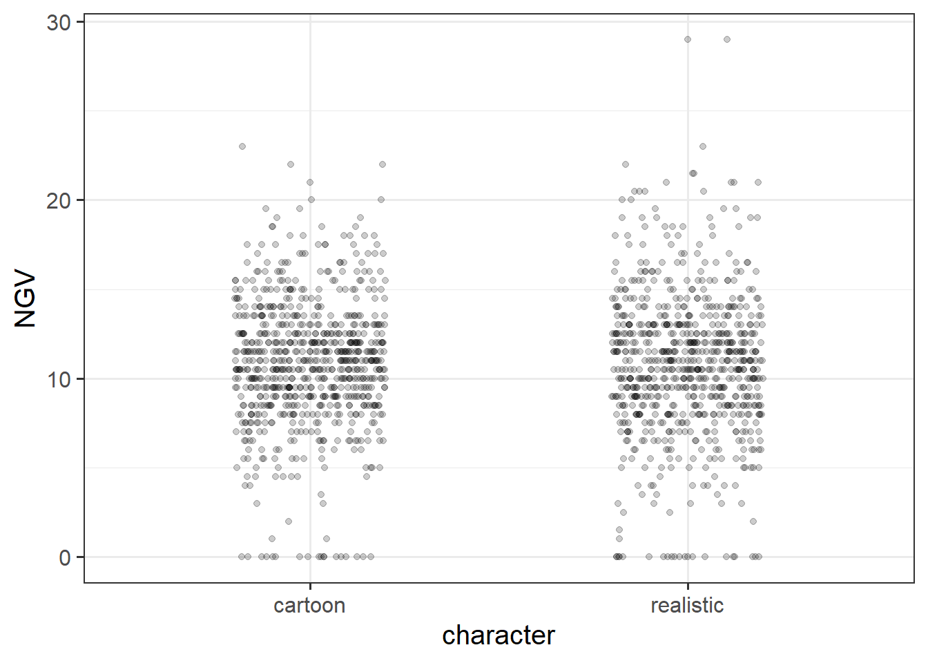
Okay. Let’s plot.. The question asks about “how the realism of video games is associated with more/less unnecessarily aggressive gameplay”.

So we’ll put the character on the x-axis and our outcome NGV on the y:
I like jitters, but you could put boxplots or violin plots too!

ggplot(ngv, aes(x = character, y = NGV)) +
  geom_jitter(height=0, width=.2, alpha=.2)

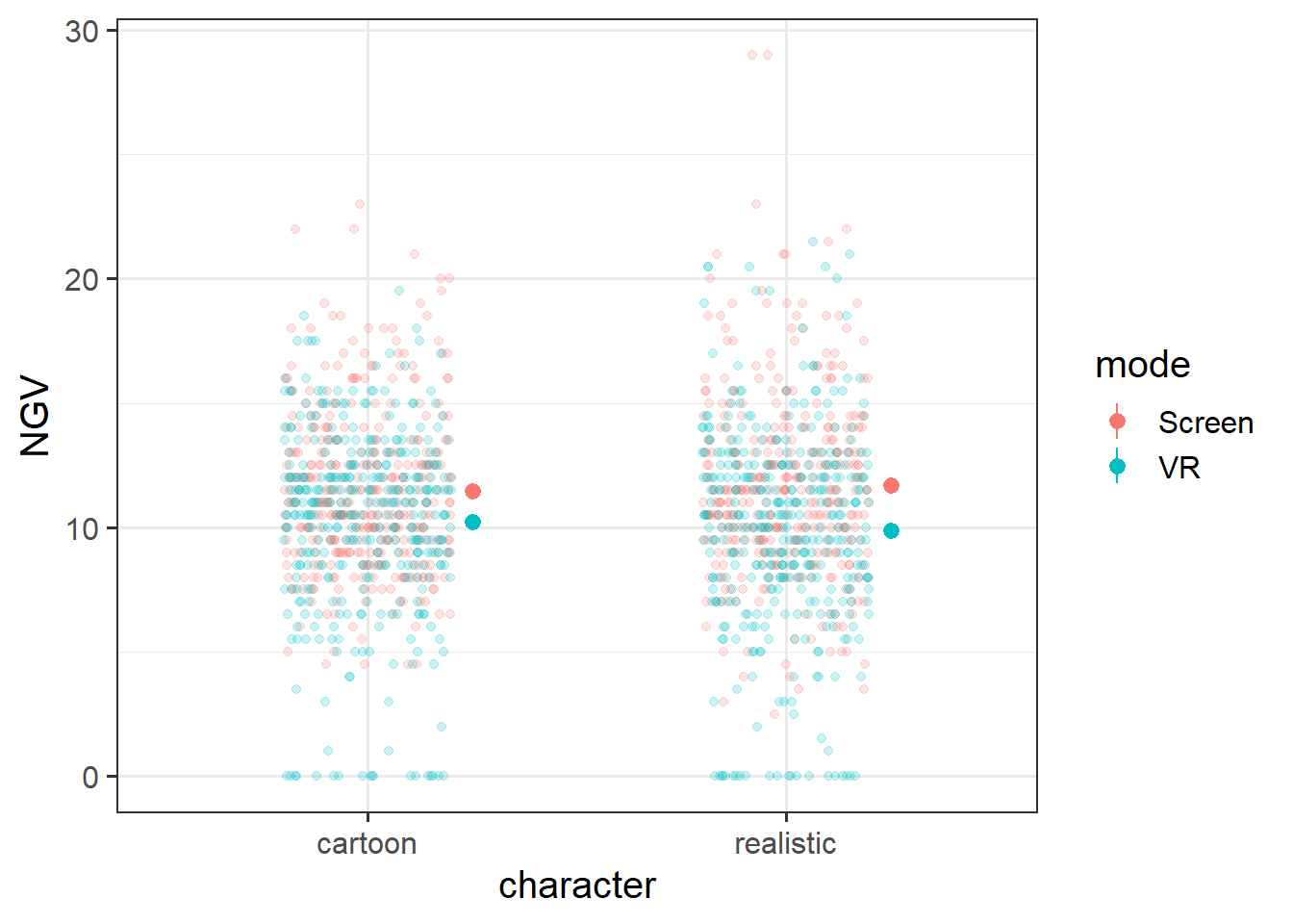
We’re also interested in whether this differs depending on the mode of gameplay (screen vs VR headset). So we could facet_wrap perhaps? or colour?
Let’s also plot the means - i’ll put those to the side of all the jittered points with a “nudge”..

ggplot(ngv, aes(x = character, y = NGV, col = mode)) +
  geom_jitter(height=0, width=.2, alpha=.2) +
  stat_summary(geom="pointrange", position = position_nudge(x=.25))

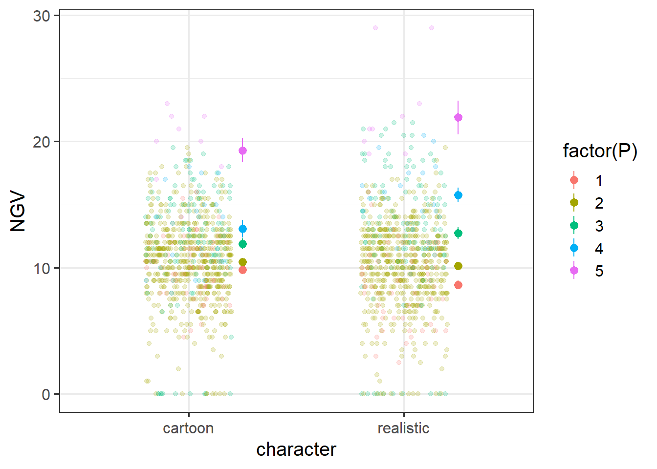
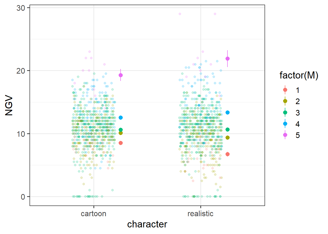
As well as looking at whether the NGV~character relationship differs between modes, we’re also interested in the differences in this relationship due to individual differences in the dark triad personality traits. We have these measured for each person, so we can just use a similar idea:

ggplot(ngv, aes(x = character, y = NGV, col = factor(P))) +
  geom_jitter(height=0, width=.2, alpha=.2) +
  stat_summary(geom="pointrange", position = position_nudge(x=.25))

ggplot(ngv, aes(x = character, y = NGV, col = factor(M))) +
  geom_jitter(height=0, width=.2, alpha=.2) +
  stat_summary(geom="pointrange", position = position_nudge(x=.25))

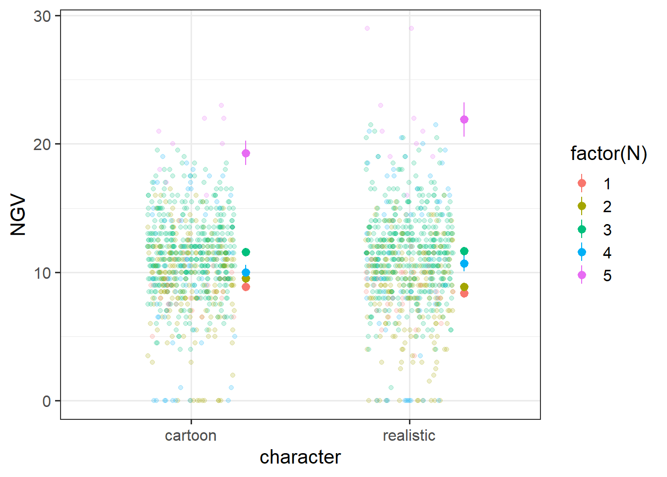
ggplot(ngv, aes(x = character, y = NGV, col = factor(N))) +
  geom_jitter(height=0, width=.2, alpha=.2) +
  stat_summary(geom="pointrange", position = position_nudge(x=.25))

What do we get from all these plots? Well, it looks like mode might be changing the relationship between character and violence. It also looks like there’s a considerable effect of the dark triad on the amount of violence people use! Of course, in these individual plots, it’s hard to ascertain the extent to which plots showing differences between levels of Narcissism are due to Narcissism or due to differences in Psychopathy (all the dark triad traits are fairly correlated)

ngv |> select(P,N,M) |>
  cor() |> round(2)
     P    N    M
P 1.00 0.43 0.51
N 0.43 1.00 0.58
M 0.51 0.58 1.00

So we need to do some modelling!

NOTE: This is how I might approach this question. There are lots of other things that we could quite sensibly do!

  • We know that we’re interested in NGV ~ character.
  • We also have the additional question of whether this is different between modes - NGV ~ character * mode.
  • And whether the NGV ~ character association is modulated by Psychopathy NGV ~ character * P, and by Narcissism NGV ~ character * N, and by Machiavellianism NGV ~ character * M.

We could fit these all in one:
NGV ~ character * (mode + P + M + N)

We have multiple observations per participant PID, and we also have multiple observations for each level level. All participants see every level, and every level is seen by all participants. It’s not the case that a level is unique to a single participant, so these are crossed.
( ?? | PID) + ( ?? | level)

Participants plays both the cartoon and the realistic versions, so we could have variation between participants in how realism affects violence - (1 + character | PID). Beyond this, all variables are measured at the participant level, so we can’t have anything else.

For the levels, each level is played by some participants in VR headsets and some participants on a screen, so we could have some levels for which VR feels very different (and makes you play more violently?) - (mode | level). We could also have some levels for which the realism has a bigger effect - (character | level), and also have some levels for which people high on the dark triad play differently - i.e. the dark triad could result in lots of violence in level 2, but not in level 3 - (P + M + N | level).

(you could also try to fit the interactions in the random effects here but i’m not going to even try!)

m0 = lmer(NGV ~ character * (mode + P + M + N) + 
            (1 + character | PID) + 
            (1 + character + mode + P + M + N | level), data = ngv)

after some simplification, I end up at the model below. You might end up at a slightly different random effect structure, and that is completely okay! The important thing is to be transparent in your decisions.

m1 = lmer(NGV ~ character * (mode + P + M + N) + 
            (1 + character | PID) + 
            (1 + mode | level), data = ngv)

Question 2

Check the assumptions of your model

We have a multilevel model, so we have assumptions at multiple levels! See 5A#mlm-assumptions-diagnostics.

Be careful - QQplots with few datapoints can make things look weirder than they are - try a histogram too

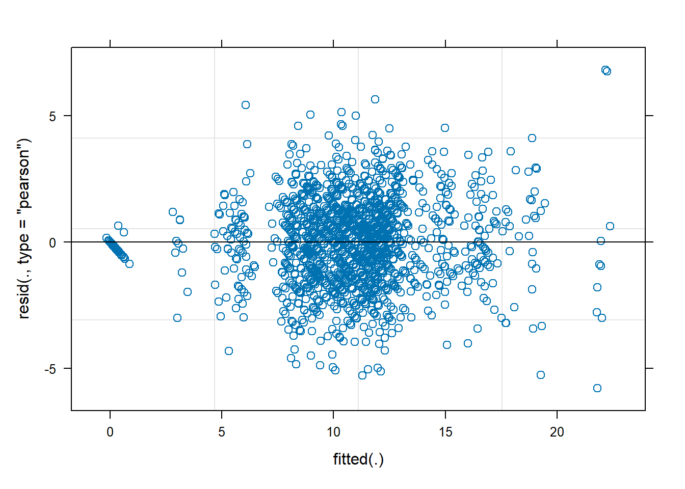
Here are some assumption plots:

plot(m1)

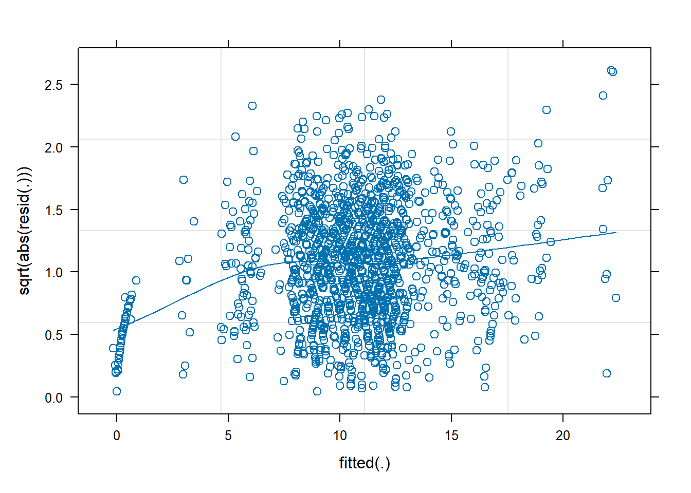
plot(m1,
     form = sqrt(abs(resid(.))) ~ fitted(.),
     type = c("p","smooth"))

There’s something weird going on in the left hand side with a bunch of points looking funny! My guess is that this may well come out when examining influence.

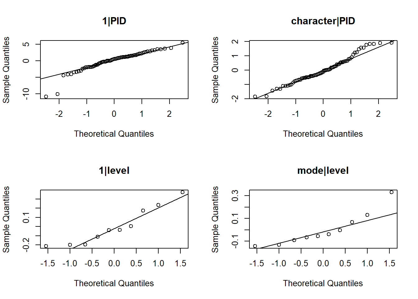
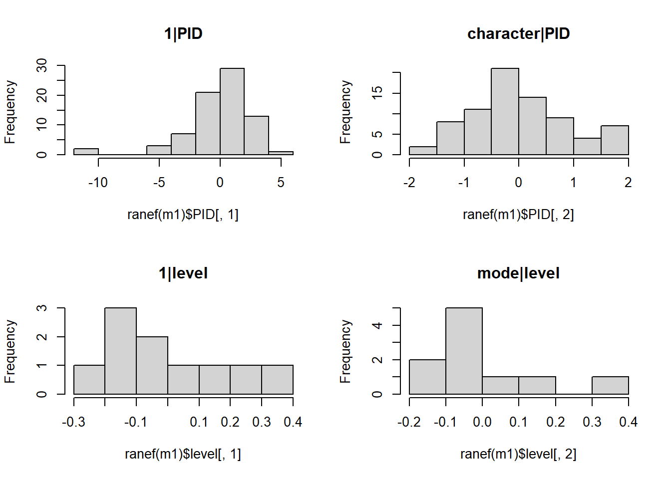
In the QQplots of the random effects below we can see a couple of participants are a bit off - this may well be what we are seeing above.

qqnorm(ranef(m1)$PID[,1],main="1|PID");qqline(ranef(m1)$PID[,1])
qqnorm(ranef(m1)$PID[,2],main="character|PID");qqline(ranef(m1)$PID[,2])
qqnorm(ranef(m1)$level[,1],main="1|level");qqline(ranef(m1)$level[,1])
qqnorm(ranef(m1)$level[,2],main="mode|level");qqline(ranef(m1)$level[,2])

The QQplots for the level random effects are hard to evaluate in part because there aren’t many levels (only 10). Let’s do some histograms too. They don’t look terrible..

hist(ranef(m1)$PID[,1],main="1|PID")
hist(ranef(m1)$PID[,2],main="character|PID")
hist(ranef(m1)$level[,1],main="1|level")
hist(ranef(m1)$level[,2],main="mode|level")

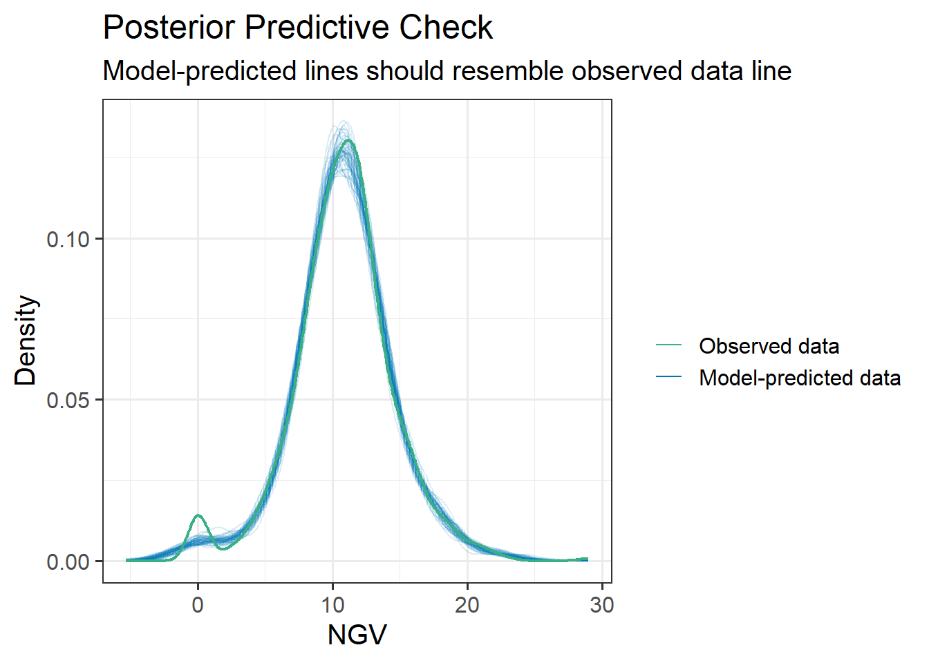
Our model predictions don’t look great either. Something is happening at values of 0?

library(performance)
check_predictions(m1)
Warning: Maximum value of original data is not included in the
  replicated data.
  Model may not capture the variation of the data.

Question 3

Check the extent to which your results may be sensitive to certain influential observations, or participants, or levels!

See 5A #influence for two packages that can assess influence.

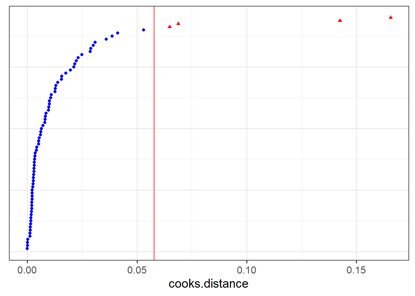
let’s check for influential participants first:

library(HLMdiag)
inf2 <- hlm_influence(m1,level="PID")
dotplot_diag(inf2$cooksd, index=inf2$PID, cutoff="internal")

and let’s re-fit without those two weird people..

m1a <- lmer(NGV ~ character * (mode + P + M + N) + 
            (1 + character | PID) + 
            (1 + mode | level), 
            data = ngv |> filter(!(PID %in% c("ppt_59","ppt_53"))))

Our conclusions change!
The significance of P (which is the association between psychopathy and needless violence in the cartoon condition) depends upon exclusion of these two participants. I’m showing the table with Satterthwaite p-values as it’s a bit quicker, but given that we have only 10 groups for the level random effect, it might be worth switching to KR

library(sjPlot)
tab_model(m1,m1a, df.method="satterthwaite")
  NGV NGV
Predictors Estimates CI p Estimates CI p
(Intercept) 6.25 3.14 – 9.35 <0.001 5.52 3.10 – 7.93 <0.001
character [realistic] -2.98 -4.48 – -1.49 <0.001 -2.98 -4.50 – -1.45 <0.001
mode [VR] -1.00 -2.34 – 0.34 0.140 -0.36 -1.41 – 0.70 0.500
P 0.90 -0.29 – 2.08 0.135 1.19 0.25 – 2.13 0.014
M 0.89 -0.20 – 1.97 0.107 0.81 -0.03 – 1.65 0.060
N 0.22 -0.90 – 1.34 0.693 0.33 -0.58 – 1.24 0.470
character [realistic] ×
mode [VR]
-0.41 -1.05 – 0.23 0.206 -0.40 -1.06 – 0.26 0.228
character [realistic] × P 0.76 0.19 – 1.33 0.010 0.79 0.19 – 1.38 0.010
character [realistic] × M 0.52 -0.00 – 1.04 0.051 0.53 -0.01 – 1.06 0.053
character [realistic] × N -0.00 -0.54 – 0.54 0.988 -0.03 -0.61 – 0.55 0.920
Random Effects
σ2 3.33 3.41
τ00 7.91 PID 4.58 PID
0.06 level 0.06 level
τ11 1.26 PID.characterrealistic 1.29 PID.characterrealistic
0.05 level.modeVR 0.05 level.modeVR
ρ01 -0.11 PID -0.18 PID
-0.51 level -0.45 level
ICC 0.71 0.59
N 76 PID 74 PID
10 level 10 level
Observations 1520 1480
Marginal R2 / Conditional R2 0.226 / 0.777 0.306 / 0.714

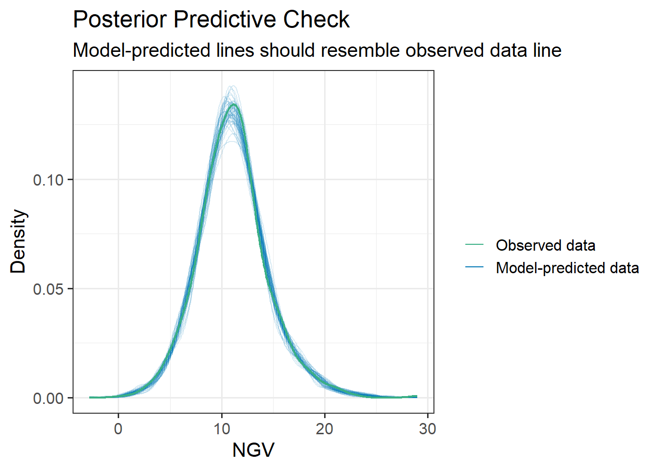
Note that our model predictions look much better

check_predictions(m1a)
Warning: Maximum value of original data is not included in the
  replicated data.
  Model may not capture the variation of the data.

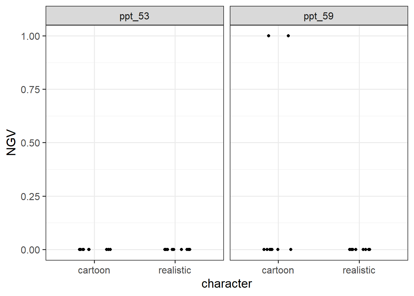
If we look at those two people - they just didn’t do much (or any) “needless game violence”.

ngv |> filter(PID %in% c("ppt_59","ppt_53")) |>
  ggplot(aes(x=character, y=NGV)) +
  geom_jitter(height=0, width=.2) + 
  facet_wrap(~PID)

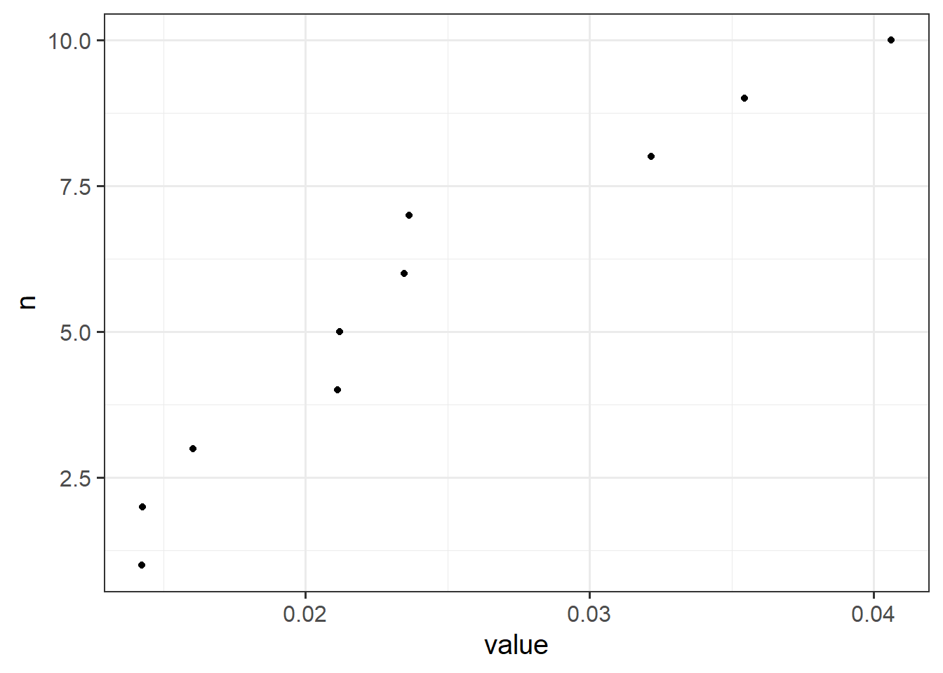
Let’s check for influential levels now:

inf3 <- hlm_influence(m1a,level="level")
dotplot_diag(inf3$cooksd)

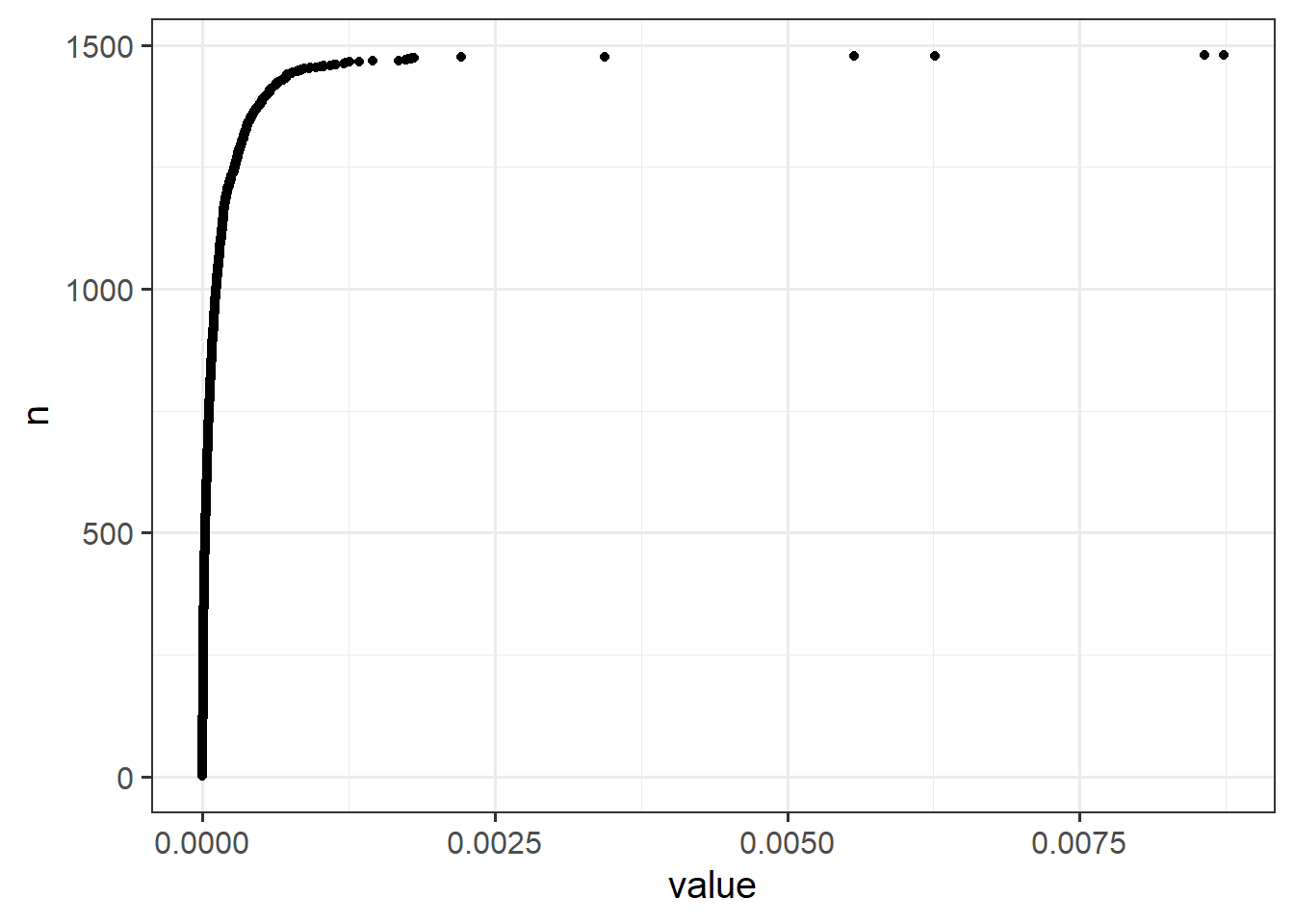
and for influential observations

inf1 <- hlm_influence(m1a,level=1)
dotplot_diag(inf1$cooksd)


All the data!

Below are all the datasets that we have seen across the readings and exercises, as well as a few extra ones that should be new! For each one, there is a quick explanation of the study design which also details the research aims of the project.

Pick one of the datasets and:

  1. explore the data, and do any required cleaning (most of them are clean already)
  2. conduct an analysis to address the research aims
  3. write a short description of the sample data (see 5B #the-sample-data)
  4. write a short explanation of your methods (see 5B #the-methods)
  5. write a short summary of your results, along with suitable visualisations and tables (see 5B #the-results)
  6. Post some of your writing on Piazza and we can collectively discuss it!

If you like, work on this as a group - set up a google doc to collaboratively write together (it’s much more fun that way!)

Readings

This dataset contains information on 900 children from 30 different schools across Scotland. The data was collected as part of a study looking at whether education-related motivation is associated with school grades. This is expected to be different for state vs privately funded schools.
All children completed an ‘education motivation’ questionnaire, and their end-of-year grade average has been recorded.

It is available at https://uoepsy.github.io/data/schoolmot.csv.

variable description
motiv Child's Education Motivation Score (range 0 - 10)
funding Funding ('state' or 'private')
schoolid Name of School that the child attends
grade Child's end-of-year grade average (0-100)
df <- read_csv("https://uoepsy.github.io/data/schoolmot.csv")

mod1 <- lmer(grade ~ motiv * funding + 
               (1 + motiv | schoolid), 
             data = df)

summary(mod1)
Linear mixed model fit by REML ['lmerMod']
Formula: grade ~ motiv * funding + (1 + motiv | schoolid)
   Data: df

REML criterion at convergence: 7083.6

Scaled residuals: 
     Min       1Q   Median       3Q      Max 
-3.08250 -0.67269  0.03043  0.63562  3.13012 

Random effects:
 Groups   Name        Variance Std.Dev. Corr 
 schoolid (Intercept) 105.126  10.253        
          motiv         2.595   1.611   -0.48
 Residual             139.030  11.791        
Number of obs: 900, groups:  schoolid, 30

Fixed effects:
                   Estimate Std. Error t value
(Intercept)         40.3143     4.6414   8.686
motiv                2.6294     0.8652   3.039
fundingstate       -17.2531     5.7347  -3.009
motiv:fundingstate   2.8485     1.0591   2.689

Correlation of Fixed Effects:
            (Intr) motiv  fndngs
motiv       -0.782              
fundingstat -0.809  0.633       
mtv:fndngst  0.639 -0.817 -0.773

Our primate researchers have been busy collecting more data. They have given a sample of Rhesus Macaques various problems to solve in order to receive treats. Troops of Macaques have a complex social structure, but adult monkeys tend can be loosely categorised as having either a “dominant” or “subordinate” status. The monkeys in our sample are either adolescent monkeys, subordinate adults, or dominant adults. Each monkey attempted various problems before they got bored/distracted/full of treats. Each problems were classed as either “easy” or “difficult”, and the researchers recorded whether or not the monkey solved each problem.

We’re interested in how the social status of monkeys is associated with the ability to solve problems.

The data is available at https://uoepsy.github.io/data/msmr_monkeystatus.csv.

variable description
status Social Status of monkey (adolescent, subordinate adult, or dominant adult)
difficulty Problem difficulty ('easy' vs 'difficult')
monkeyID Monkey Name
solved Whether or not the problem was successfully solved by the monkey
df <- read_csv("https://uoepsy.github.io/data/msmr_monkeystatus.csv")

# relevel difficulty
df$difficulty <- factor(df$difficulty, 
                        levels=c("easy","difficult"))

mod1 <- glmer(solved ~ difficulty + status +
                (1 + difficulty | monkeyID), 
              family=binomial,
              data = df)

summary(mod1)
Generalized linear mixed model fit by maximum likelihood (Laplace
  Approximation) [glmerMod]
 Family: binomial  ( logit )
Formula: solved ~ difficulty + status + (1 + difficulty | monkeyID)
   Data: df

     AIC      BIC   logLik deviance df.resid 
   503.7    531.6   -244.8    489.7      390 

Scaled residuals: 
    Min      1Q  Median      3Q     Max 
-1.9358 -0.6325 -0.3975  0.6748  2.5160 

Random effects:
 Groups   Name                Variance Std.Dev. Corr 
 monkeyID (Intercept)         1.551    1.246         
          difficultydifficult 1.371    1.171    -0.44
Number of obs: 397, groups:  monkeyID, 50

Fixed effects:
                    Estimate Std. Error z value Pr(>|z|)   
(Intercept)          -0.3945     0.3867  -1.020  0.30767   
difficultydifficult  -0.8586     0.3053  -2.812  0.00492 **
statusdominant        0.6682     0.4714   1.417  0.15637   
statussubordinate     1.4596     0.5692   2.564  0.01033 * 
---
Signif. codes:  0 '***' 0.001 '**' 0.01 '*' 0.05 '.' 0.1 ' ' 1

Correlation of Fixed Effects:
            (Intr) dffclt sttsdm
dffcltydffc -0.333              
statusdmnnt -0.721 -0.031       
statssbrdnt -0.594 -0.033  0.497

A study is interested in examining whether engaging in mindfulness can prevent cognitive decline in older adults. They recruit a sample of 20 participants at age 60, and administer the Addenbrooke’s Cognitive Examination (ACE) every 2 years (until participants were aged 78). Half of the participants complete weekly mindfulness sessions, while the remaining participants did not.

The data are available at: https://uoepsy.github.io/data/msmr_mindfuldecline.csv.

variable description
ppt Participant Identifier
condition Whether the participant engages in mindfulness or not (control/mindfulness)
study_visit Study Visit Number (1 - 10)
age Age (in years) at study visit
ACE Addenbrooke's Cognitive Examination Score. Scores can range from 0 to 100
imp Clinical diagnosis of cognitive impairment ('imp' = impaired, 'unimp' = unimpaired)
df <- read_csv("https://uoepsy.github.io/data/msmr_mindfuldecline.csv")

#recenter age
df$ageC <- df$age-60

mod1 <- lmer(ACE ~ 1 + ageC * condition + 
               (1 + ageC | ppt), 
             data = df)

summary(mod1)
Linear mixed model fit by REML ['lmerMod']
Formula: ACE ~ 1 + ageC * condition + (1 + ageC | ppt)
   Data: df

REML criterion at convergence: 365

Scaled residuals: 
     Min       1Q   Median       3Q      Max 
-2.29607 -0.68577 -0.04105  0.68630  2.42029 

Random effects:
 Groups   Name        Variance Std.Dev. Corr
 ppt      (Intercept) 0.11982  0.3462       
          ageC        0.01923  0.1387   0.26
 Residual             0.24453  0.4945       
Number of obs: 177, groups:  ppt, 20

Fixed effects:
                          Estimate Std. Error t value
(Intercept)               85.20343    0.14927 570.796
ageC                      -0.26595    0.04483  -5.933
conditionmindfulness       0.04803    0.20871   0.230
ageC:conditionmindfulness  0.17294    0.06343   2.726

Correlation of Fixed Effects:
            (Intr) ageC   cndtnm
ageC         0.068              
cndtnmndfln -0.715 -0.048       
agC:cndtnmn -0.048 -0.707  0.073

Previous research has evidenced a notable dip in happiness for middle-aged humans. Interestingly, this phenomenon has even been observed in other primates, such as chimpanzees.

The present study is interested in examining whether the ‘middle-age slump’ happens to a similar extent for Orangutans as it does for Chimpanzees.

0 apes (0 Chimps and 0 Orangutans) were included in the study. All apes were studied from early adulthood (10-12 years old for most great apes), and researchers administered the Happiness in Primates (HiP) scale to each participant every 3 years, up until the age of 40.

The data are available at https://uoepsy.github.io/data/midlife_ape.csv.

The dataset has already been cleaned, and the researchers have confirmed that it includes 0 Chimps and 0 Orangutans, and every ape has complete data (i.e. 10 rows for each ape).

variable description
apeID Ape's Name (all names are chosen to be unique)
age Age (in years) at assessment
species Species (chimp v orangutan)
HiP Happiness in Primate Scale (range 1 to 18)
timepoint Study visit (1 to 10)
df <- read_csv("https://uoepsy.github.io/data/midlife_ape.csv")

# add polynomials
df <- df |> 
  mutate(
    poly1 = poly(timepoint,2,raw=F)[,1],
    poly2 = poly(timepoint,2,raw=F)[,2]
  )

mod1 = lmer(HiP ~ 1 + (poly1 + poly2) * species +
            (1 + poly1 + poly2 | apeID), 
            data = df)

summary(mod1)
Linear mixed model fit by REML ['lmerMod']
Formula: HiP ~ 1 + (poly1 + poly2) * species + (1 + poly1 + poly2 | apeID)
   Data: df

REML criterion at convergence: 6908.3

Scaled residuals: 
    Min      1Q  Median      3Q     Max 
-3.1222 -0.6175  0.0017  0.6340  3.2438 

Random effects:
 Groups   Name        Variance Std.Dev. Corr     
 apeID    (Intercept)   4.346   2.085            
          poly1        27.673   5.261   0.11     
          poly2       106.915  10.340   0.10 0.52
 Residual               1.247   1.117            
Number of obs: 2000, groups:  apeID, 200

Fixed effects:
                       Estimate Std. Error t value
(Intercept)              9.1155     0.1955  46.630
poly1                    1.8796     1.5391   1.221
poly2                    9.4004     1.7453   5.386
speciesorangutan         0.6853     0.3035   2.258
poly1:speciesorangutan   0.1104     2.3892   0.046
poly2:speciesorangutan  -6.2718     2.7093  -2.315

Correlation of Fixed Effects:
            (Intr) poly1  poly2  spcsrn ply1:s
poly1        0.033                            
poly2        0.054  0.090                     
specisrngtn -0.644 -0.021 -0.035              
ply1:spcsrn -0.021 -0.644 -0.058  0.033       
ply2:spcsrn -0.035 -0.058 -0.644  0.054  0.090

Suppose that we conducted an experiment on a sample of 20 staff members from the Psychology department to investigate effects of CBD consumption on stress over the course of the working week. Participants were randomly allocated to one of two conditions: the control group continued as normal, and the CBD group were given one CBD drink every day. Over the course of the working week (5 days) participants stress levels were measured using a self-report questionnaire.

Dataset: https://uoepsy.github.io/data/stressweek1.csv.

variable description
dept Department
pid Participant Name
CBD Whether or not they were allocated to the control group (N) or the CBD group (Y)
measure Measure used to assess stress levels
day Day of the working week (1 to 5)
stress Stress Level (standardised)
df <- read_csv("https://uoepsy.github.io/data/stressweek1.csv")
# re-center 'day' so the intercept is day 1
df$day <- df$day-1 

mod1 <- lmer(stress ~ 1 + day * CBD + 
               (1 + day | pid), 
             data = df)

summary(mod1)
Linear mixed model fit by REML ['lmerMod']
Formula: stress ~ 1 + day * CBD + (1 + day | pid)
   Data: df

REML criterion at convergence: 127.7

Scaled residuals: 
     Min       1Q   Median       3Q      Max 
-2.17535 -0.65204 -0.02667  0.64622  1.81574 

Random effects:
 Groups   Name        Variance Std.Dev. Corr
 pid      (Intercept) 0.199441 0.44659      
          day         0.004328 0.06579  0.02
 Residual             0.112462 0.33535      
Number of obs: 100, groups:  pid, 20

Fixed effects:
            Estimate Std. Error t value
(Intercept)  0.13178    0.14329   0.920
day          0.07567    0.03461   2.186
CBDY        -0.08516    0.24221  -0.352
day:CBDY    -0.19128    0.05851  -3.270

Correlation of Fixed Effects:
         (Intr) day    CBDY  
day      -0.339              
CBDY     -0.592  0.201       
day:CBDY  0.201 -0.592 -0.339

As for previous study, but instead of a sample of 20 participants from the psychology staff, we have 240 people from various departments such as History, Philosophy, Art, etc..

Dataset: https://uoepsy.github.io/data/stressweek_nested.csv.

variable description
dept Department
pid Participant Name
CBD Whether or not they were allocated to the control group (N) or the CBD group (Y)
measure Measure used to assess stress levels
day Day of the working week (1 to 5)
stress Stress Level (standardised)
df <- read_csv("https://uoepsy.github.io/data/stressweek_nested.csv")

# re-center 'day' so the intercept is day 1
df$day <- df$day-1 

# removed day*CBD|dept to obtain convergence
mod1 <- lmer(stress ~ 1 + day * CBD + 
               (1 + day + CBD | dept) +
               (1 + day | dept:pid), 
             data = df)

summary(mod1)
Linear mixed model fit by REML ['lmerMod']
Formula: stress ~ 1 + day * CBD + (1 + day + CBD | dept) + (1 + day |  
    dept:pid)
   Data: df

REML criterion at convergence: 1681.7

Scaled residuals: 
    Min      1Q  Median      3Q     Max 
-2.9964 -0.5700  0.0014  0.5790  2.7610 

Random effects:
 Groups   Name        Variance Std.Dev. Corr       
 dept:pid (Intercept) 0.14768  0.38430             
          day         0.01214  0.11019  -0.03      
 dept     (Intercept) 0.64863  0.80538             
          day         0.00198  0.04449  -0.18      
          CBDY        0.05534  0.23524   0.40 -0.22
 Residual             0.12976  0.36023             
Number of obs: 1200, groups:  dept:pid, 240; dept, 12

Fixed effects:
            Estimate Std. Error t value
(Intercept)  0.03888    0.23724   0.164
day          0.07651    0.02002   3.821
CBDY        -0.10608    0.09380  -1.131
day:CBDY    -0.13900    0.02115  -6.572

Correlation of Fixed Effects:
         (Intr) day    CBDY  
day      -0.165              
CBDY      0.182  0.040       
day:CBDY  0.052 -0.572 -0.245

As for version 1 of this study (20 staff members from the Psychology department), but instead of taking a measurement only on a self-report scale, we took 10 different measures every time point (cortisol levels, blood pressure, heart rate variability, various questionnaires etc).

Dataset: https://uoepsy.github.io/data/stressweek_crossed.csv

variable description
dept Department
pid Participant Name
CBD Whether or not they were allocated to the control group (N) or the CBD group (Y)
measure Measure used to assess stress levels
day Day of the working week (1 to 5)
stress Stress Level (standardised)
df <- read_csv("https://uoepsy.github.io/data/stressweek_crossed.csv")

# re-center 'day' so the intercept is day 1
df$day <- df$day-1 

# removed day*CBD|dept to obtain convergence
mod1 <- lmer(stress ~ 1 + day * CBD + 
                (1 + day + CBD | measure) +
                (1 + day | pid), 
             data = df)

summary(mod1)
Linear mixed model fit by REML ['lmerMod']
Formula: stress ~ 1 + day * CBD + (1 + day + CBD | measure) + (1 + day |  
    pid)
   Data: df

REML criterion at convergence: 670.5

Scaled residuals: 
     Min       1Q   Median       3Q      Max 
-2.86174 -0.66229  0.09594  0.68404  2.42687 

Random effects:
 Groups   Name        Variance Std.Dev. Corr       
 pid      (Intercept) 0.261627 0.51149             
          day         0.014693 0.12121  -0.32      
 measure  (Intercept) 0.143948 0.37940             
          day         0.008543 0.09243   0.93      
          CBDY        0.283487 0.53244  -0.05  0.11
 Residual             0.088073 0.29677             
Number of obs: 1000, groups:  pid, 20; measure, 10

Fixed effects:
            Estimate Std. Error t value
(Intercept) -0.08096    0.18689  -0.433
day          0.12651    0.04530   2.793
CBDY        -0.15808    0.29498  -0.536
day:CBDY    -0.25830    0.05850  -4.415

Correlation of Fixed Effects:
         (Intr) day    CBDY  
day       0.187              
CBDY     -0.390  0.167       
day:CBDY  0.154 -0.452 -0.279

Labs

Recall the example from last semesters’ USMR course, where the lectures explored linear regression with a toy dataset of how practice influences the reading age of toy characters (see USMR Week 7 Lecture). We’re going to now broaden our scope to the investigation of how practice affects reading age for all toys (not just Martin’s Playmobil characters).

You can find a dataset at https://uoepsy.github.io/data/toy2.csv containing information on 129 different toy characters that come from a selection of different families/types of toy.

variable description
toy_type Type of Toy
year Year Released
toy Character
hrs_week Hours of practice per week
R_AGE Reading Age

This data is from a simulated study that aims to investigate the following research question:

How do different types of audio interfere with executive functioning, and does this interference differ depending upon whether or not noise-cancelling headphones are used?

30 healthy volunteers each completed the Symbol Digit Modalities Test (SDMT) - a commonly used test to assess processing speed and motor speed - a total of 15 times. During the tests, participants listened to either no audio (5 tests), white noise (5 tests) or classical music (5 tests). Half the participants listened via active-noise-cancelling headphones, and the other half listened via speakers in the room. Unfortunately, lots of the tests were not administered correctly, and so not every participant has the full 15 trials worth of data.

The data is available at https://uoepsy.github.io/data/efsdmt.csv.

variable description
PID Participant ID
audio Audio heard during the test ('no_audio', 'white_noise','music')
headphones Whether the participant listened via speakers in the room or via noise cancelling headphones
SDMT Symbol Digit Modalities Test (SDMT) score

We have data from a large sample of great apes who have been studied between the ages of 1 to 10 years old (i.e. during adolescence). Our data includes 4 species of great apes: Chimpanzees, Bonobos, Gorillas and Orangutans. Each ape has been assessed on a primate dominance scale at various ages. Data collection was not very rigorous, so apes do not have consistent assessment schedules (i.e., one may have been assessed at ages 1, 3 and 6, whereas another at ages 2 and 8).

The researchers are interested in examining how the adolescent development of dominance in great apes differs between species.

Data on the dominance scores of the apes are available at https://uoepsy.github.io/data/msmr_apeage.csv and the information about which species each ape is are in https://uoepsy.github.io/data/msmr_apespecies.csv.

Table 1:

Data Dictionary: msmr_apespecies.csv

variable description
ape Ape Name
species Species (Bonobo, Chimpanzee, Gorilla, Orangutan)
Table 2:

Data Dictionary: msmr_apeage.csv

variable description
ape Ape Name
age Age at assessment (years)
dominance Dominance (Z-scored)

The “Trolley Problem” is a thought experiment in moral philosophy that asks you to decide whether or not to pull a lever to divert a trolley. Pulling the lever changes the trolley direction from hitting 5 people to a track on which it will hit one person.
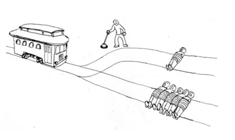
Previous research has found that the “framing” of the problem will influence the decisions people make:

positive frame neutral frame negative frame
5 people will be saved if you pull the lever; one person on another track will be saved if you do not pull the lever. All your actions are legal and understandable. Will you pull the lever? 5 people will be saved if you pull the lever, but another person will die. One people will be saved if you do not pull the lever, but 5 people will die. All your actions are legal and understandable. Will you pull the lever? One person will die if you pull the lever. 5 people will die if you do not pull the lever. All your actions are legal and understandable. Will you pull the lever?

We conducted a study to investigate whether the framing effects on moral judgements depends upon the stakes (i.e. the number of lives saved).

120 participants were recruited, and each gave answers to 12 versions of the thought experiment. For each participant, four versions followed each of the positive/neutral/negative framings described above, and for each framing, 2 would save 5 people and 2 would save 15 people.

The data are available at https://uoepsy.github.io/data/msmr_trolley.csv.

variable description
PID Participant ID
frame framing of the thought experiment (positive/neutral/negative
lives lives at stake in the thought experiment (5 or 15)
lever Whether or not the participant chose to pull the lever (1 = yes, 0 = no)
load(url("https://uoepsy.github.io/msmr/data/nwl.RData"))

In the nwl data set (accessed using the code above), participants with aphasia are separated into two groups based on the general location of their brain lesion: anterior vs. posterior. There is data on the numbers of correct and incorrect responses participants gave in each of a series of experimental blocks. There were 7 learning blocks, immediately followed by a test. Finally, participants also completed a follow-up test.
Data were also collect from healthy controls.
Figure 1 shows the differences between lesion location groups in the average proportion of correct responses at each point in time (i.e., each block, test, and follow-up)
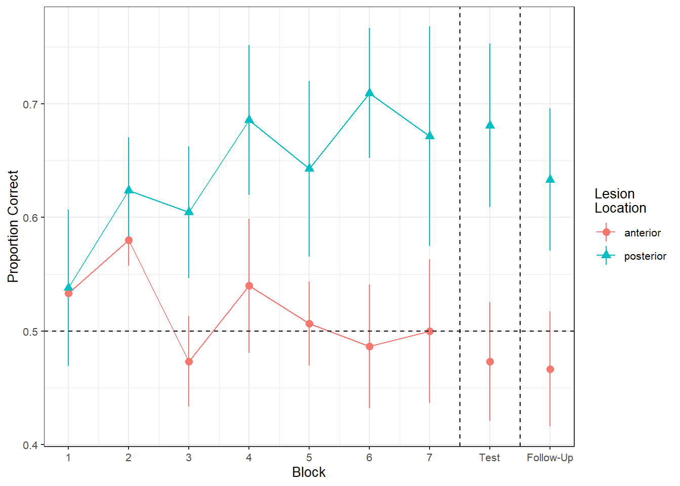
Figure 1: Differences between groups in the average proportion of correct responses at each block
variable description
group Whether participant is a stroke patient ('patient') or a healthy control ('control')
lesion_location Location of brain lesion: anterior vs posterior
block Experimental block (1-9). Blocks 1-7 were learning blocks, immediately followed by a test in block 8. Block 9 was a follow-up test at a later point
PropCorrect Proportion of 30 responses in a given block that the participant got correct
NumCorrect Number of responses (out of 30) in a given block that the participant got correct
NumError Number of responses (out of 30) in a given block that the participant got incorrect
ID Participant Identifier
Phase Experimental phase, corresponding to experimental block(s): 'Learning', 'Immediate','Follow-up'

These data are available at https://uoepsy.github.io/data/Az.rda. You can load the dataset using:

load(url("https://uoepsy.github.io/data/Az.rda"))

and you will find the Az object in your environment.

The Az object contains information on 30 Participants with probable Alzheimer’s Disease, who completed 3 tasks over 10 time points: A memory task, and two scales investigating ability to undertake complex activities of daily living (cADL) and simple activities of daily living (sADL). Performance on all of tasks was calculated as a percentage of total possible score, thereby ranging from 0 to 100.

We’re interested in whether performance on these tasks differed at the outset of the study, and if they differed in their subsequent change in performance.

variable description
Subject Unique Subject Identifier
Time Time point of the study (1 to 10)
Task Task type (Memory, cADL, sADL)
Performance Score on test (range 0 to 100)

This is synthetic data from a randomised controlled trial, in which 30 therapists randomly assigned patients (each therapist saw between 4 and 30 patients) to a control or treatment group, and monitored their scores over time on a measure of generalised anxiety disorder (GAD7 - a 7 item questionnaire with 5 point likert scales).

The control group of patients received standard sessions offered by the therapists. For the treatment group, 10 mins of each sessions was replaced with a specific psychoeducational component, and patients were given relevant tasks to complete between each session. All patients had monthly therapy sessions. Generalised Anxiety Disorder was assessed at baseline and then every visit over 4 months of sessions (5 assessments in total).

The data are available at https://uoepsy.github.io/data/msmr_gadeduc.csv

You can find a data dictionary below:

variable description
patient A patient code in which the labels take the form <Therapist initials>_<group>_<patient number>.
visit_0 Score on the GAD7 at baseline
visit_1 GAD7 at 1 month assessment
visit_2 GAD7 at 2 month assessment
visit_3 GAD7 at 3 month assessment
visit_4 GAD7 at 4 month assessment

An experiment was run to conceptually replicate “test-enhanced learning” (Roediger & Karpicke, 2006): two groups of 25 participants were presented with material to learn. One group studied the material twice (StudyStudy), the other group studied the material once then did a test (StudyTest). Recall was tested immediately (one minute) after the learning session and one week later. The recall tests were composed of 175 items identified by a keyword (Test_word).

The critical (replication) prediction is that the StudyStudy group recall more items on the immediate test, but the StudyTest group will retain the material better and thus perform better on the 1-week follow-up test.

The following code loads the data into your R environment by creating a variable called tel:

load(url("https://uoepsy.github.io/data/testenhancedlearning.RData"))
variable description
Subject_ID Unique Participant Identifier
Group Group denoting whether the participant studied the material twice (StudyStudy), or studied it once then did a test (StudyTest)
Delay Time of recall test ('min' = Immediate, 'week' = One week later)
Test_word Word being recalled (175 different test words)
Correct Whether or not the word was correctly recalled
Rtime Time to recall word (milliseconds)

488 children from 30 schools were included in the study. Children were assessed on a yearly basis for 7 years throughout primary school on a measure of vocabulary administered in English, the Picture Vocab Test (PVT). 295 were monolingual English speakers, and 193 were bilingual (english + another language).

Previous research conducted on monolingual children has suggested that that scores on the PVT increase steadily up until the age of approximately 7 or 8 at which point they begin to plateau. The aim of the present study is to investigate differences in the development of vocabulary between monolingual and bilingual children.

The data are available at https://uoepsy.github.io/data/pvt_bilingual.csv.

variable description
child Child's name
school School Identifier
isBilingual Binary variable indicating whether the child is monolingual (0) or bilingual (1)
age Age (years)
PVT Score on the Picture Vocab Test (PVT). Scores range 0 to 60

New

Are children with more day-to-day routine better at regulating their emotions? A study of 200 children from 20 schools (9 private schools and 11 state schools) completed a survey containing the Emotion Dysregulation Scale (EDS) and the Child Routines Questionnaire (CRQ).

DATASET: https://uoepsy.github.io/data/crqeds.csv

variable description
schoolid School Identifier
EDS Emotion Dysregulation Score (range 1-6, higher values indicate more *dys*regulation of emotions)
CRQ Childhood Routine Questionnaire Score (range 0-7, higher values indicate more day-to-day routine)
schooltype School type (private / state)
df <- read_csv("https://uoepsy.github.io/data/crqeds.csv")

mod1 <- lmer(EDS ~ schooltype + CRQ + 
       (1 + CRQ | schoolid), 
       data = df)

summary(mod1)
Linear mixed model fit by REML ['lmerMod']
Formula: EDS ~ schooltype + CRQ + (1 + CRQ | schoolid)
   Data: df

REML criterion at convergence: 289.4

Scaled residuals: 
     Min       1Q   Median       3Q      Max 
-1.85256 -0.84640  0.02332  0.66027  2.04265 

Random effects:
 Groups   Name        Variance Std.Dev. Corr 
 schoolid (Intercept) 0.20734  0.4553        
          CRQ         0.01891  0.1375   -0.76
 Residual             0.23942  0.4893        
Number of obs: 174, groups:  schoolid, 20

Fixed effects:
                Estimate Std. Error t value
(Intercept)      4.53262    0.17583  25.778
schooltypeState -0.16708    0.15415  -1.084
CRQ             -0.05306    0.05067  -1.047

Correlation of Fixed Effects:
            (Intr) schltS
scholtypStt -0.510       
CRQ         -0.762  0.042

Does clothing seem more attractive to shoppers when it is viewed on a model, and is this dependent on item price? 30 participants were presented with a set of pictures of items of clothing, and rated each item how likely they were to buy it. Each participant saw 20 items, ranging in price from £5 to £100. 15 participants saw these items worn by a model, while the other 15 saw the items against a white background.

DATASET: https://uoepsy.github.io/data/dapr3_mannequin.csv

variable description
purch_rating Purchase Rating (sliding scale 0 to 100, with higher ratings indicating greater perceived likelihood of purchase)
price Price presented with item (range £5 to £100)
ppt Participant Identifier
condition Whether items are seen on a model or on a white background
df <- read_csv("https://uoepsy.github.io/data/dapr3_mannequin.csv")

#scale price to help convergence
#change 1 in price is now change of £10
df$price <- df$price/10

mod1 <- lmer(purch_rating ~ price*condition + 
       (1+price|ppt), 
       data = df)
  
summary(mod1)
Linear mixed model fit by REML ['lmerMod']
Formula: purch_rating ~ price * condition + (1 + price | ppt)
   Data: df

REML criterion at convergence: 4754.6

Scaled residuals: 
    Min      1Q  Median      3Q     Max 
-3.7237 -0.6389  0.0491  0.6836  3.2354 

Random effects:
 Groups   Name        Variance Std.Dev. Corr 
 ppt      (Intercept)  59.361   7.7046       
          price         0.713   0.8444  -0.78
 Residual             148.039  12.1671       
Number of obs: 600, groups:  ppt, 30

Fixed effects:
                     Estimate Std. Error t value
(Intercept)           41.2807     2.4672  16.732
price                  2.4767     0.3270   7.575
conditionmodel        -1.8533     3.4891  -0.531
price:conditionmodel   1.1600     0.4624   2.509

Correlation of Fixed Effects:
            (Intr) price  cndtnm
price       -0.804              
conditinmdl -0.707  0.568       
prc:cndtnmd  0.568 -0.707 -0.804

Researchers want to study the relationship between time spent outdoors and mental wellbeing, across all of Scotland. They contact all the Local Authority Areas (LAAs) and ask them to collect data for them, with participants completing the Warwick-Edinburgh Mental Wellbeing Scale (WEMWBS), a self-report measure of mental health and well-being, and being asked to estimate the average number of hours they spend outdoors each week. Twenty of the Local Authority Areas provided data.

DATASET: https://uoepsy.github.io/data/LAAwellbeing.csv

variable description
ppt Participant Identifier
name Participant Name
laa Local Authority Area
outdoor_time Number of hours spent outdoors per week
wellbeing Wellbeing score (Warwick Edinburgh Mental Wellbeing Scale). Range 15 - 75, with higher scores indicating better mental wellbeing
density Population density of local authority area (number of people per square km)
df <- read_csv("https://uoepsy.github.io/data/LAAwellbeing.csv")

mod1 <- lmer(wellbeing ~ density + outdoor_time + 
       (1 + outdoor_time | laa), 
       data = df) 

summary(mod1)
Linear mixed model fit by REML ['lmerMod']
Formula: wellbeing ~ density + outdoor_time + (1 + outdoor_time | laa)
   Data: df

REML criterion at convergence: 863.8

Scaled residuals: 
     Min       1Q   Median       3Q      Max 
-2.25154 -0.55979  0.00415  0.62341  1.95652 

Random effects:
 Groups   Name         Variance Std.Dev. Corr
 laa      (Intercept)  53.1785  7.2924       
          outdoor_time  0.1095  0.3309   0.14
 Residual              21.3433  4.6199       
Number of obs: 132, groups:  laa, 20

Fixed effects:
              Estimate Std. Error t value
(Intercept)  39.123896   2.289384  17.089
density      -0.002121   0.002234  -0.949
outdoor_time  0.216197   0.102358   2.112

Correlation of Fixed Effects:
            (Intr) densty
density     -0.445       
outdoor_tim -0.291  0.025

easter egg: check for influential people!

The “Wellbeing in Work” dataset contains information on employee wellbeing, assessed at baseline (start of study), 12 months post, 24 months post, and 36 months post. over the course of 36 months. Participants were randomly assigned to one of three employment conditions:

  • control: No change to employment. Employees continue at 5 days a week, with standard allocated annual leave quota.
  • unlimited_leave : Employees were given no limit to their annual leave, but were still expected to meet required targets as specified in their job description.
  • fourday_week: Employees worked a 4 day week for no decrease in pay, and were still expected to meet required targets as specified in their job description.

The researchers have two main questions: Overall, did the participants’ wellbeing stay the same or did it change? Did the employment condition groups differ in the how wellbeing changed over the assessment period?

DATASET: https://uoepsy.github.io/data/wellbeingwork3.rda

variable description
ID Participant ID
TimePoint Timepoint (0 = baseline, 1 = 12 months, 2 = 24 months, 3 = 36 months)
Condition Employment Condition ('control' = 5 day week, 28 days of leave. 'unlimited_leave' = 5 days a week, unlimited leave. 'fourday_week' = 4 day week, 28 days of leave)
Wellbeing Wellbeing score (Warwick Edinburgh Mental Wellbeing Scale). Range 15 - 75, with higher scores indicating better mental wellbeing
load(url("https://uoepsy.github.io/data/wellbeingwork3.rda"))

mod1 <- lmer(Wellbeing~TimePoint+(1+TimePoint|ID), 
             data = wellbeingwork3)
mod2 <- lmer(Wellbeing~TimePoint+Condition+(1+TimePoint|ID), 
             data = wellbeingwork3)
mod3 <- lmer(Wellbeing~TimePoint*Condition+(1+TimePoint|ID), 
             data = wellbeingwork3)
anova(mod1,mod2,mod3)
Data: wellbeingwork3
Models:
mod1: Wellbeing ~ TimePoint + (1 + TimePoint | ID)
mod2: Wellbeing ~ TimePoint + Condition + (1 + TimePoint | ID)
mod3: Wellbeing ~ TimePoint * Condition + (1 + TimePoint | ID)
     npar    AIC    BIC  logLik deviance  Chisq Df Pr(>Chisq)    
mod1    6 4171.7 4199.2 -2079.8   4159.7                         
mod2    8 4164.3 4200.9 -2074.2   4148.3 11.393  2   0.003358 ** 
mod3   10 4144.6 4190.4 -2062.3   4124.6 23.711  2  7.098e-06 ***
---
Signif. codes:  0 '***' 0.001 '**' 0.01 '*' 0.05 '.' 0.1 ' ' 1
summary(mod3)
Linear mixed model fit by REML ['lmerMod']
Formula: Wellbeing ~ TimePoint * Condition + (1 + TimePoint | ID)
   Data: wellbeingwork3

REML criterion at convergence: 4127.5

Scaled residuals: 
     Min       1Q   Median       3Q      Max 
-3.02242 -0.56063 -0.01029  0.59140  3.09484 

Random effects:
 Groups   Name        Variance Std.Dev. Corr 
 ID       (Intercept)  0.8077  0.8987        
          TimePoint    3.8622  1.9653   -0.71
 Residual             12.3969  3.5209        
Number of obs: 720, groups:  ID, 180

Fixed effects:
                                   Estimate Std. Error t value
(Intercept)                        38.35167    0.39761  96.456
TimePoint                          -0.02333    0.32511  -0.072
Conditionunlimited_leave           -0.01833    0.56230  -0.033
Conditionfourday_week              -0.26000    0.56230  -0.462
TimePoint:Conditionunlimited_leave  1.35667    0.45977   2.951
TimePoint:Conditionfourday_week     2.28167    0.45977   4.963

Correlation of Fixed Effects:
              (Intr) TimPnt Cndtnn_ Cndtnf_ TmPnt:Cndtnn_
TimePoint     -0.642                                     
Cndtnnlmtd_   -0.707  0.454                              
Cndtnfrdy_w   -0.707  0.454  0.500                       
TmPnt:Cndtnn_  0.454 -0.707 -0.642  -0.321               
TmPnt:Cndtnf_  0.454 -0.707 -0.321  -0.642   0.500       

In 2010 A US state’s commissioner for education was faced with growing community concern about rising levels of adolescent antisocial behaviours.

After a series of focus groups, the commissioner approved the trialing of an intervention in which yearly Parent Management Training (PMT) group sessions were offered to the parents of a cohort of students entering 10 different high schools. Every year, the parents were asked to fill out an informant-based version of the Aggressive Behaviour Scale (ABS), measuring verbal and physical abuse, socially inappropriate behavior, and resisting care. Where possible, the same parents were followed up throughout the child’s progression through high school. Alongside this, parents from a cohort of students entering 10 further high schools in the state were recruited to also complete the same informant-based ABS, but were not offered the PMT group sessions.
The commissioner has two main questions: Does the presentation of aggressive behaviours increase as children enter the secondary school system? If so, is there any evidence for the effectiveness of Parent Management Training (PMT) group sessions in curbing the rise of aggressive behaviors during a child’s transition into the secondary school system?

DATASET: https://uoepsy.github.io/data/abs_intervention.csv

variable description
schoolid School Name
ppt Participant Identifier
age Age (years)
interv Whether or not parents attended Parent Management Training (PMT) group sessions (0 = No, 1 = Yes)
ABS Aggressive Behaviours Scale. Measures verbal and physical abuse, socially inappropriate behavior, and resisting care. Scores range from 0 to 100, with higher scores indicating more aggressive behaviours.

Check here: https://uoepsy.github.io/dapr3/2324/lectures/dapr3_2324_05b_rq2mod.html#4

These data are simulated to represent data from a fake experiment, in which participants were asked to drive around a route in a 30mph zone. Each participant completed the route 3 times (i.e. “repeated measures”), but each time they were listening to different audio (either speech, classical music or rap music). Their average speed across the route was recorded. This is a fairly simple design, that we might use to ask “how is the type of audio being listened to associated with driving speeds?”

The data are available at https://uoepsy.github.io/data/drivingmusicwithin.csv.

variable description
pid Participant Identifier
speed Avg Speed Driven on Route (mph)
music Music listened to while driving (classical music / rap music / spoken word)
df <- read_csv("https://uoepsy.github.io/data/drivingmusicwithin.csv")

Temptation is to fit the below, but it won’t work, because each pid has only 1 obs for each music, so we’re overfitting

mod1 <- lmer(speed ~ music + 
               (1 + music | pid), 
             data = df)
Error: number of observations (=150) <= number of random effects (=150) for term (1 + music | pid); the random-effects parameters and the residual variance (or scale parameter) are probably unidentifiable
mod1 <- lmer(speed ~ music + 
               (1 | pid), 
             data = df)

summary(mod1)
Linear mixed model fit by REML ['lmerMod']
Formula: speed ~ music + (1 | pid)
   Data: df

REML criterion at convergence: 895.5

Scaled residuals: 
     Min       1Q   Median       3Q      Max 
-2.47567 -0.56300 -0.01549  0.54691  2.42387 

Random effects:
 Groups   Name        Variance Std.Dev.
 pid      (Intercept) 20.32    4.508   
 Residual             13.54    3.679   
Number of obs: 150, groups:  pid, 50

Fixed effects:
            Estimate Std. Error t value
(Intercept)  34.2456     0.8229  41.615
musicrap     -5.7905     0.7358  -7.869
musicspeech  -5.2048     0.7358  -7.073

Correlation of Fixed Effects:
            (Intr) muscrp
musicrap    -0.447       
musicspeech -0.447  0.500

These data are simulated to represent data from 50 participants, each measured at 3 different time-points (pre, during, and post) on a measure of stress. Participants were randomly allocated such that half received some cognitive behavioural therapy (CBT) treatment, and half did not. This study is interested in assessing whether the two groups (control vs treatment) differ in how stress changes across the 3 time points.

The data are available at https://uoepsy.github.io/data/stressint.csv.

variable description
ppt Participant Identifier
stress Stress (range 0 to 100)
time Time (pre/post/during)
group Whether participant is in the CBT group or control group
df <- read_csv("https://uoepsy.github.io/data/stressint.csv")
df$time <- factor(df$time, levels=c("Pre","During","Post"))

Temptation is to fit the below, but it won’t work, because each pid has only 1 obs for each music, so we’re overfitting

mod1 <- lmer(stress ~ time*group + 
               (1 + time|ppt), 
             data = df)
Error: number of observations (=150) <= number of random effects (=150) for term (1 + time | ppt); the random-effects parameters and the residual variance (or scale parameter) are probably unidentifiable
mod1 <- lmer(stress ~ time*group + 
               (1 |ppt), 
             data = df)

summary(mod1)
Linear mixed model fit by REML ['lmerMod']
Formula: stress ~ time * group + (1 | ppt)
   Data: df

REML criterion at convergence: 1096.5

Scaled residuals: 
     Min       1Q   Median       3Q      Max 
-1.83946 -0.53326 -0.05639  0.53766  2.31546 

Random effects:
 Groups   Name        Variance Std.Dev.
 ppt      (Intercept) 184.82   13.595  
 Residual              43.26    6.577  
Number of obs: 150, groups:  ppt, 50

Fixed effects:
                          Estimate Std. Error t value
(Intercept)                 62.840      3.020  20.805
timeDuring                  -3.200      1.860  -1.720
timePost                    -6.760      1.860  -3.634
groupTreatment               1.920      4.272   0.449
timeDuring:groupTreatment  -21.120      2.631  -8.028
timePost:groupTreatment    -28.440      2.631 -10.810

Correlation of Fixed Effects:
            (Intr) tmDrng timPst grpTrt tmDr:T
timeDuring  -0.308                            
timePost    -0.308  0.500                     
groupTrtmnt -0.707  0.218  0.218              
tmDrng:grpT  0.218 -0.707 -0.354 -0.308       
tmPst:grpTr  0.218 -0.354 -0.707 -0.308  0.500

These data are simulated to represent data from 30 participants who took part in an experiment designed to investigate whether fluency of speech influences how believable an utterance is perceived to be.

Each participant listened to the same 20 statements, with 10 being presented in fluent speech, and 10 being presented with a disfluency (an “erm, …”). Fluency of the statements was counterbalanced such that 15 participants heard statements 1 to 10 as fluent and 11 to 20 as disfluent, and the remaining 15 participants heard statements 1 to 10 as disfluent, and 11 to 20 as fluent. The order of the statements presented to each participant was random. Participants rated each statement on how believable it is on a scale of 0 to 100.

The data are available at https://uoepsy.github.io/data/erm_belief.csv.

variable description
ppt Participant Identifier
trial_n Trial number
sentence Statement identifier
condition Condition (fluent v disfluent)
belief belief rating (0-100)
statement Statement
df <- read_csv("https://uoepsy.github.io/data/erm_belief.csv")
# make trial_n numeric
df$trial_n <- as.numeric(gsub("trial_","",df$trial_n))
# relevel condition:
df$condition <- factor(df$condition, levels=c("fluent","disfluent"))

# having (trial_n | ppt) doesn't converge, so simplify to:
mod1 <- lmer(belief ~ trial_n + condition + 
               (1 | ppt) + 
               (1 + condition | statement), 
             data = df)

summary(mod1)
Linear mixed model fit by REML ['lmerMod']
Formula: belief ~ trial_n + condition + (1 | ppt) + (1 + condition | statement)
   Data: df

REML criterion at convergence: 3732.4

Scaled residuals: 
    Min      1Q  Median      3Q     Max 
-2.7869 -0.6440 -0.0320  0.6498  3.4210 

Random effects:
 Groups    Name               Variance Std.Dev. Corr 
 ppt       (Intercept)         0.7144  0.8452        
 statement (Intercept)         6.0925  2.4683        
           conditiondisfluent  2.8453  1.6868   -0.09
 Residual                     26.3688  5.1351        
Number of obs: 600, groups:  ppt, 30; statement, 20

Fixed effects:
                   Estimate Std. Error t value
(Intercept)        49.80050    0.74668  66.696
trial_n            -0.04966    0.03716  -1.337
conditiondisfluent -2.02893    0.56469  -3.593

Correlation of Fixed Effects:
            (Intr) tril_n
trial_n     -0.503       
cndtndsflnt -0.227 -0.051

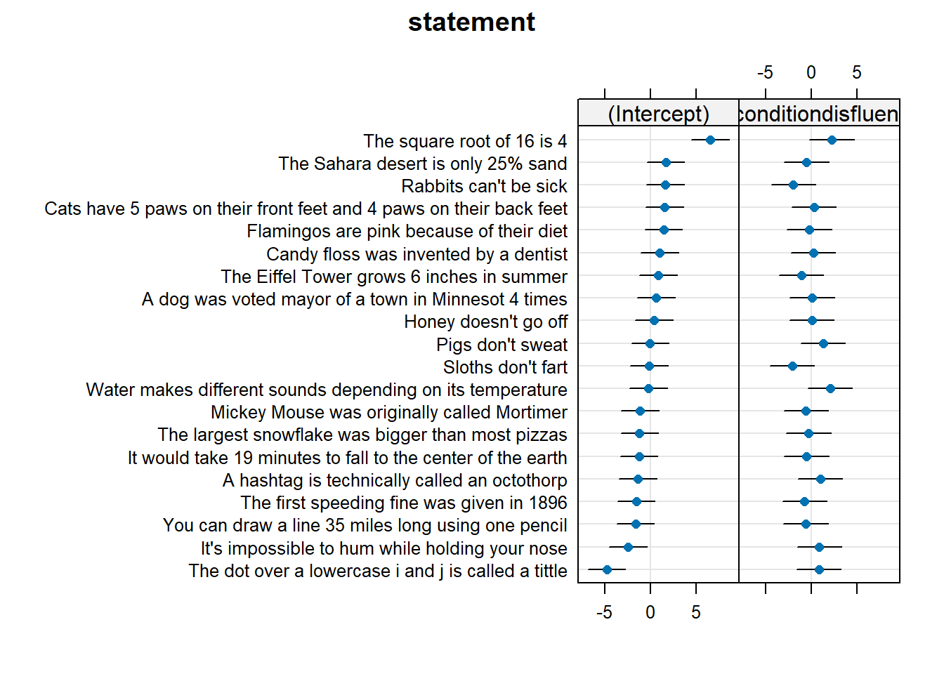
easter egg: plot your ranefs

dotplot.ranef.mer(ranef(mod1))$statement

These data are simulated to represent a large scale international study of cognitive aging, for which data from 17 research centers has been combined. The study team are interested in whether different cognitive domains have different trajectories as people age. Do all cognitive domains decline at the same rate? Do some decline more steeply, and some less? The literature suggests that scores on cognitive ability are predicted by educational attainment, so they would like to control for this.

Each of the 17 research centers recruited a minimum of 14 participants (Median = 21, Range 14-29) at age 48, and recorded their level of education (in years). Participants were then tested on 5 cognitive domains: processing speed, spatial visualisation, memory, reasoning, and vocabulary. Participants were contacted for follow-up on a further 9 occasions (resulting in 10 datapoints for each participant), and at every follow-up they were tested on the same 5 cognitive domains. Follow-ups were on average 3 years apart (Mean = 3, SD = 0.8).

The data are available at https://uoepsy.github.io/data/cogdecline.csv.

variable description
cID Center ID
pptID Participant Identifier
educ Educational attainment (years of education)
age Age at visit (years)
processing_speed Score on Processing Speed domain task
spatial_visualisation Score on Spatial Visualisation domain task
memory Score on Memory domain task
reasoning Score on Reasoning domain task
vocabulary Score on Vocabulary domain task
df <- read_csv("https://uoepsy.github.io/data/cogdecline.csv")

# reshape
df <- df |> pivot_longer(processing_speed:vocabulary,
                   names_to = "domain",
                   values_to = "score")

# recenter age and educ
df$age <- df$age - 48
df$educ <- df$educ - min(df$educ)

this won’t converge:

mod1 <- lmer(score ~ educ + age * domain + 
               (1 + educ + age * domain | cID) + 
               (1 + age * domain | cID:pptID),
             data = df)
mod1 <- lmer(score ~ educ + age * domain + 
               (1 | cID) + 
               (1 + age | cID:pptID) +
               (1 | cID:pptID:domain),
             data = df,
             control=lmerControl(optimizer="bobyqa"))

summary(mod1)
Linear mixed model fit by REML ['lmerMod']
Formula: score ~ educ + age * domain + (1 | cID) + (1 + age | cID:pptID) +  
    (1 | cID:pptID:domain)
   Data: df
Control: lmerControl(optimizer = "bobyqa")

REML criterion at convergence: 82497

Scaled residuals: 
    Min      1Q  Median      3Q     Max 
-3.7903 -0.6569  0.0085  0.6598  3.9712 

Random effects:
 Groups           Name        Variance Std.Dev. Corr
 cID:pptID:domain (Intercept) 0.06134  0.2477       
 cID:pptID        (Intercept) 1.74032  1.3192       
                  age         0.01047  0.1023   0.26
 cID              (Intercept) 0.03628  0.1905       
 Residual                     4.01099  2.0027       
Number of obs: 18950, groups:  cID:pptID:domain, 1895; cID:pptID, 379; cID, 17

Fixed effects:
                                 Estimate Std. Error t value
(Intercept)                     -1.203378   0.240409  -5.006
educ                             0.293357   0.036099   8.126
age                             -0.024486   0.006466  -3.787
domainprocessing_speed           0.080018   0.087180   0.918
domainreasoning                  0.063089   0.087180   0.724
domainspatial_visualisation      0.020739   0.087180   0.238
domainvocabulary                -0.779985   0.087180  -8.947
age:domainprocessing_speed      -0.005106   0.005326  -0.959
age:domainreasoning             -0.001689   0.005326  -0.317
age:domainspatial_visualisation -0.001290   0.005326  -0.242
age:domainvocabulary             0.064308   0.005326  12.074

Correlation of Fixed Effects:
            (Intr) educ   age    dmnpr_ dmnrsn dmnsp_ dmnvcb ag:dmnp_ ag:dmnr
educ        -0.904                                                           
age         -0.063  0.000                                                    
dmnprcssng_ -0.181  0.000  0.339                                             
domainrsnng -0.181  0.000  0.339  0.500                                      
dmnsptl_vsl -0.181  0.000  0.339  0.500  0.500                               
domanvcblry -0.181  0.000  0.339  0.500  0.500  0.500                        
ag:dmnprcs_  0.149  0.000 -0.412 -0.824 -0.412 -0.412 -0.412                 
ag:dmnrsnng  0.149  0.000 -0.412 -0.412 -0.824 -0.412 -0.412  0.500          
ag:dmnsptl_  0.149  0.000 -0.412 -0.412 -0.412 -0.824 -0.412  0.500    0.500 
ag:dmnvcblr  0.149  0.000 -0.412 -0.412 -0.412 -0.412 -0.824  0.500    0.500 
            ag:dmns_
educ                
age                 
dmnprcssng_         
domainrsnng         
dmnsptl_vsl         
domanvcblry         
ag:dmnprcs_         
ag:dmnrsnng         
ag:dmnsptl_         
ag:dmnvcblr  0.500