Week 1 Exercises: Intro to MLM

New Packages!

These are the main packages we’re going to use in this block. It might make sense to install them now if you do not have them already

• tidyverse : for organising data
  
• lme4 : for fitting generalised linear mixed effects models
• broom.mixed : tidying methods for mixed models
• effects : for tabulating and graphing effects in linear models
• lmerTest: for quick p-values from mixed models
• parameters: various inferential methods for mixed models

A Toy Example

For our first foray into the multilevel model, we’re going to start with little toy example, and we’re just going to ask you to plot the predictions from a) a simple linear model, b) a model with a random intercept, and c) a model with random intercepts and slopes.

This is to build the understanding of the structure of multilevel models. When it comes to actually building models for research purposes, it is not necessary to slowly build up the complexity in this way.

Data: New Toys!

Recall the example from last semesters’ USMR course, where the lectures explored linear regression with a toy dataset of how practice influences the reading age of toy characters (see USMR Week 7 Lecture). We’re going to now broaden our scope to the investigation of how practice affects reading age for all toys (not just Martin’s Playmobil characters).

You can find a dataset at https://uoepsy.github.io/data/toy2.csv containing information on 129 different toy characters that come from a selection of different families/types of toy. You can see the variables in the table below¹.

variable	description
toy_type	Type of Toy
year	Year Released
toy	Character
hrs_week	Hours of practice per week
R_AGE	Reading Age

Question 1

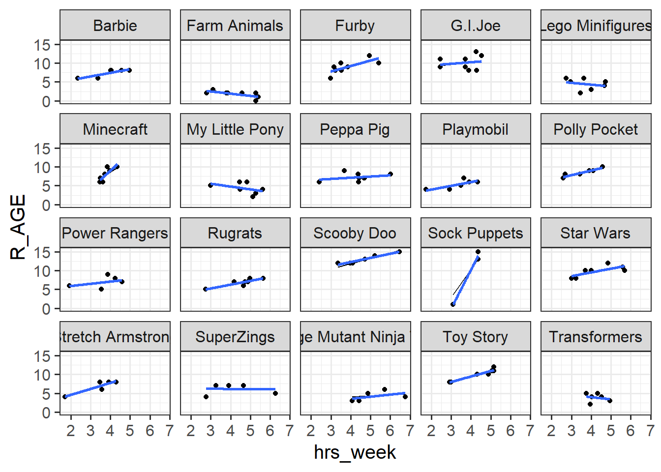
Read in the data and plot the relationship between hours-per-week practice (hrs_week) and reading age (R_AGE).
Facet the plot by the type of toy.

Hints

“facet” is the key word here! See 1A #visualisations

library(tidyverse)
toy2 <- read_csv("https://uoepsy.github.io/data/toy2.csv")

head(toy2)

# A tibble: 6 × 5
  toy_type  year toy    hrs_week R_AGE
  <chr>    <dbl> <chr>     <dbl> <dbl>
1 Barbie    1959 Summer     4.04     8
2 Barbie    1959 Nikki      2.36     6
3 Barbie    1959 Barbie     4.02     8
4 Barbie    1959 Midge      4.97     8
5 Barbie    1959 Teresa     3.37     6
6 Barbie    1959 Ken        4.56     8

ggplot(toy2,aes(x=hrs_week,y=R_AGE))+
  geom_point()+
  facet_wrap(~toy_type)

Question 2

Below is the code to fit a simple linear model and produce some diagnostic plots.
After running the code, do you think that we have violated any assumptions?

mod1 <- lm(R_AGE ~ hrs_week, data = toy2)
plot(mod1)

We have violated an assumption here, and we don’t need to look at the plots to realise it! As it happens, the plots don’t actually look terrible (the scale-location plot is a bit meh, but other than that things look okay).

The assumption we have violated is that of independence. This is something we know through our understanding of the sampling procedure that has led to this data. We have got a random sample of different types of toys (e.g. power-rangers, toy-story, furbies etc), and within those types, we have a random sample of characters.

But it is entirely likely that the type of toy is going to influence their reading age (i.e. farm animals might read worse than playmobil, etc).

So this is something we can’t really “see” in the data - we have to think. What do we know about the data generating process? (i.e. the process that led to this data)

mod1 <- lm(R_AGE ~ hrs_week, data = toy2)
plot(mod1)

Question 3

There are lots of ways in R to get predicted values for a linear model (e.g. we saw augment() a lot in USMR).

The simplest way is to use functions like predict() or fitted() (they do the same thing), which gives us a vector of predicted values, which we can append to our dataframe (provided we don’t have missing data):

data$predictedvalues <- predict(model)

Add the predictions from the linear model in the previous question to the facetted plot that you created in the earlier question. How well does the model fit each type of toy?

This only works because we don’t have missing data (and so the length of predict(mod1) is the same as nrow(toy2), and the predictions are in the correct order)

# add predictions to data:
toy2$pred <- predict(mod1)

# plot both predictions and observations:
toy2 |>
  ggplot(aes(x=hrs_week))+
  geom_point(aes(y=R_AGE)) + # observations
  geom_line(aes(y=pred)) + # predictions
  facet_wrap(~toy_type)

Question 4

Load the lme4 package, and fit a model with random intercepts for each toy type.

Using either predict() again, or this time you can use augment() from the broom.mixed package, plot the predicted values and the observations.

Hints

You can see a model with a random intercept fitted in 1B# fitting-multilevel-models-in-r.

Here’s our model, with a random intercept by toy-type:

library(lme4)
library(broom.mixed)

mod2 <- lmer(R_AGE ~ 1 + hrs_week + (1 | toy_type), data = toy2)

We can use augment() from the broom.mixed package, and which gives us the variables in the model along with things like fitted values (in the .fitted column)

augment(mod2)

# A tibble: 129 × 14
  R_AGE hrs_week toy_type .fitted  .resid  .hat  .cooksd .fixed   .mu .offset
  <dbl>    <dbl> <fct>      <dbl>   <dbl> <dbl>    <dbl>  <dbl> <dbl>   <dbl>
1     8     4.04 Barbie      7.43  0.574  0.158 0.0144     7.14  7.43       0
2     6     2.36 Barbie      6.23 -0.229  0.183 0.00282    5.94  6.23       0
3     8     4.02 Barbie      7.41  0.587  0.158 0.0151     7.12  7.41       0
4     8     4.97 Barbie      8.09 -0.0855 0.170 0.000354   7.80  8.09       0
5     6     3.37 Barbie      6.95 -0.950  0.161 0.0404     6.66  6.95       0
# ℹ 124 more rows
# ℹ 4 more variables: .sqrtXwt <dbl>, .sqrtrwt <dbl>, .weights <dbl>,
#   .wtres <dbl>

augment(mod2) |>
  ggplot(aes(x=hrs_week))+
  geom_point(aes(y=R_AGE)) + # observations
  geom_line(aes(y=.fitted)) + # predictions
  facet_wrap(~toy_type)

Note that the model predictions are now a lot better than they were for the single level linear model. The line has moved up for the “Scooby Doos”, and down for the “Farm Animals”, etc. But the lines are all still the same slope. The slope is “fixed”.

Question 5

Now fit a model with random intercepts and slopes for each toy type.

As before, plot the predicted values of this model alongside the observations

mod3 <- lmer(R_AGE ~ 1 + hrs_week + (1 + hrs_week| toy_type), 
             data = toy2)

augment(mod3) |>
  ggplot(aes(x=hrs_week))+
  geom_point(aes(y=R_AGE)) + # observations
  geom_line(aes(y=.fitted)) + # predictions
  facet_wrap(~toy_type)

This looks even better - the lines are at good heights and good angles for each type of toy. Why? Because we have modelled the intercept (line height) and slope of hrs_week (line angle) as varying across types of toy!

Question 6

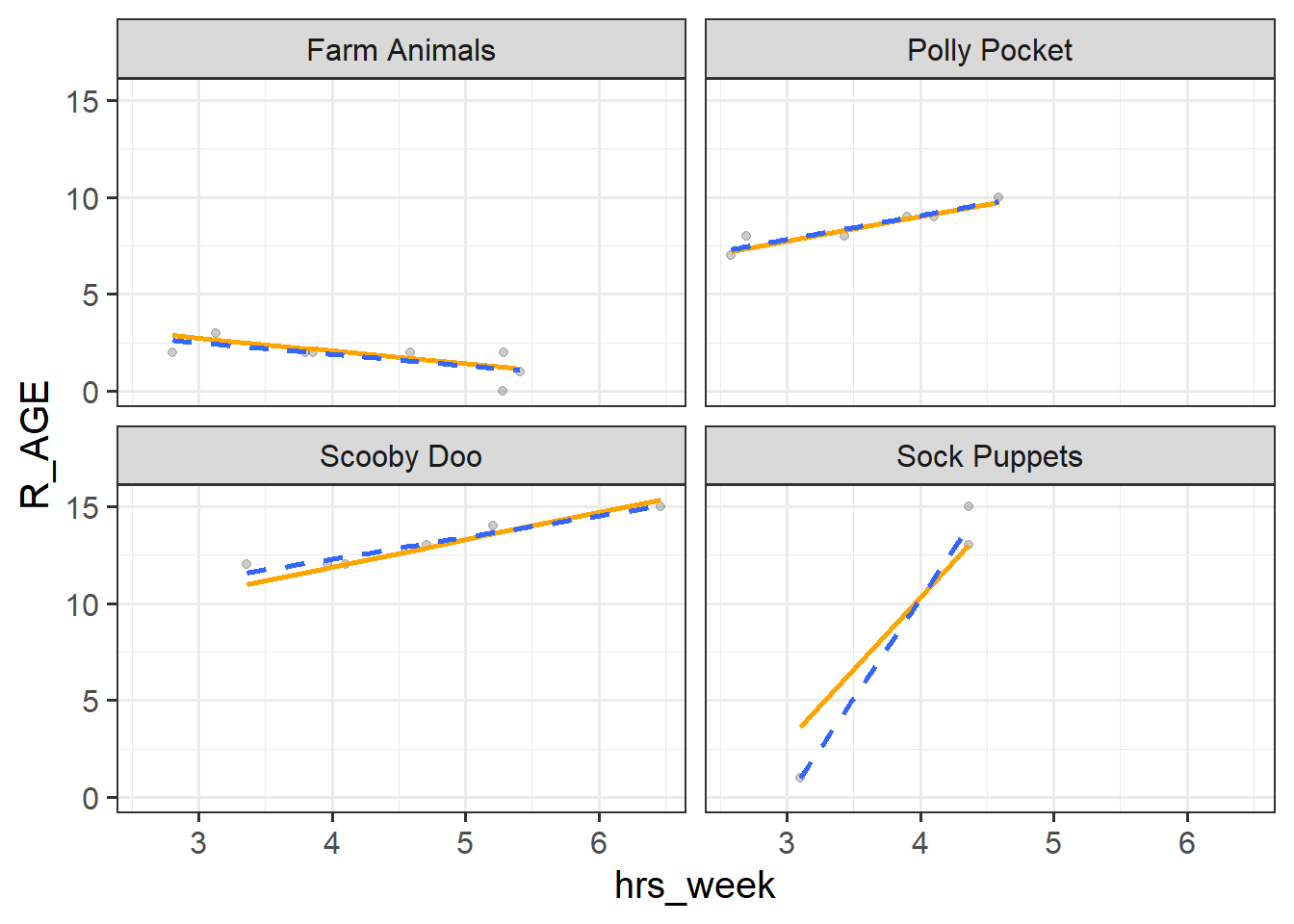
Finally, add a geom_smooth to the plot from the previous question (making sure that this is has y=R_AGE).
This will add a separate linear model lm() line for each of the facets in the plot.

What differences (look closely!) do you notice between the predictions from the model with random intercepts and slopes, and the simple geom_smooths?

Hints

You could try changing col, lty, and lwd to make things easier to see.

What we’re doing here is showing to ourselves ‘partial pooling’ in action (1B #partial-pooling).

here’s the model we are using:

mod3 <- lmer(R_AGE ~ 1 + hrs_week + (1 + hrs_week| toy_type), 
             data = toy2)

and here is our plot:

augment(mod3) |>
  ggplot(aes(x=hrs_week))+
  geom_point(aes(y=R_AGE)) + # observations
  geom_line(aes(y=.fitted)) + # predictions
  geom_smooth(aes(y=R_AGE), method=lm, se=F) + # simple smooths
  facet_wrap(~toy_type)

I’ve made it a bit clearer here by changing up the colours and linewidths (lwd), and subsetting to just a select few of the toy types:

augment(mod3) |>
  filter(toy_type %in% c("Farm Animals","Scooby Doo","Sock Puppets","Polly Pocket")) |>
  ggplot(aes(x=hrs_week))+
  geom_point(aes(y=R_AGE), alpha=.2) + # observations
  geom_line(aes(y=.fitted), col="orange", lwd=1) + # predictions
  geom_smooth(aes(y=R_AGE), method=lm, se=F, lty="dashed") + # simple smooths
  facet_wrap(~toy_type)

For most of the toy types things look pretty similar. However, for “Sock Puppets” (only has 3 data points) the model predicted slope is shrunk back towards the average. It is also possible to see this in the “Farm Animals” and “Scooby Doo” - the shrinkage is more noticeable on these because they are further away from the average.

Question 7

Here is the model with the random intercepts (but not random slopes) that we fitted in an earlier question.

Below is the code that produces a plot of the fitted values:

A. Model Equation

$$ \[\begin{align} \text{For Toy }j\text{ of Type }i & \\ \text{Level 1 (Toy):}& \\ \text{R\_AGE}_{ij} &= b_{0i} + b_1 \cdot \text{hrs\_week}_{ij} + \epsilon_{ij} \\ \text{Level 2 (Type):}& \\ b_{0i} &= \gamma_{00} + \zeta_{0i} \\ \text{Where:}& \\ \zeta_{0i} &\sim N(0,\sigma_{0}) \\ \varepsilon &\sim N(0,\sigma_{e}) \\ \end{align}\]

$$

B. Model output

mod2 <- lmer(R_AGE ~ 1 + hrs_week + (1 | toy_type), 
             data = toy2)
summary(mod2)

Linear mixed model fit by REML ['lmerMod']
Formula: R_AGE ~ 1 + hrs_week + (1 | toy_type)
   Data: toy2

REML criterion at convergence: 544.7

Scaled residuals: 
    Min      1Q  Median      3Q     Max 
-4.8809 -0.4687  0.0541  0.5579  3.3220 

Random effects:
 Groups   Name        Variance Std.Dev.
 toy_type (Intercept) 7.278    2.698   
 Residual             2.550    1.597   
Number of obs: 129, groups:  toy_type, 20

Fixed effects:
            Estimate Std. Error t value
(Intercept)   4.2594     0.9157   4.652
hrs_week      0.7118     0.1651   4.312

Correlation of Fixed Effects:
         (Intr)
hrs_week -0.736

C. Plot of fitted values

augment(mod2) |>
  ggplot(aes(x=hrs_week, col=toy_type))+
  geom_point(aes(y=R_AGE),alpha=.3) + # observations
  geom_line(aes(y=.fitted)) + # predictions 
  geom_abline(intercept = fixef(mod2)[1], 
              slope = fixef(mod2)[2], lwd=1) +  # fixed effect line
  guides(col="none") + # remove legend
  xlim(0,7) # extent to x=0

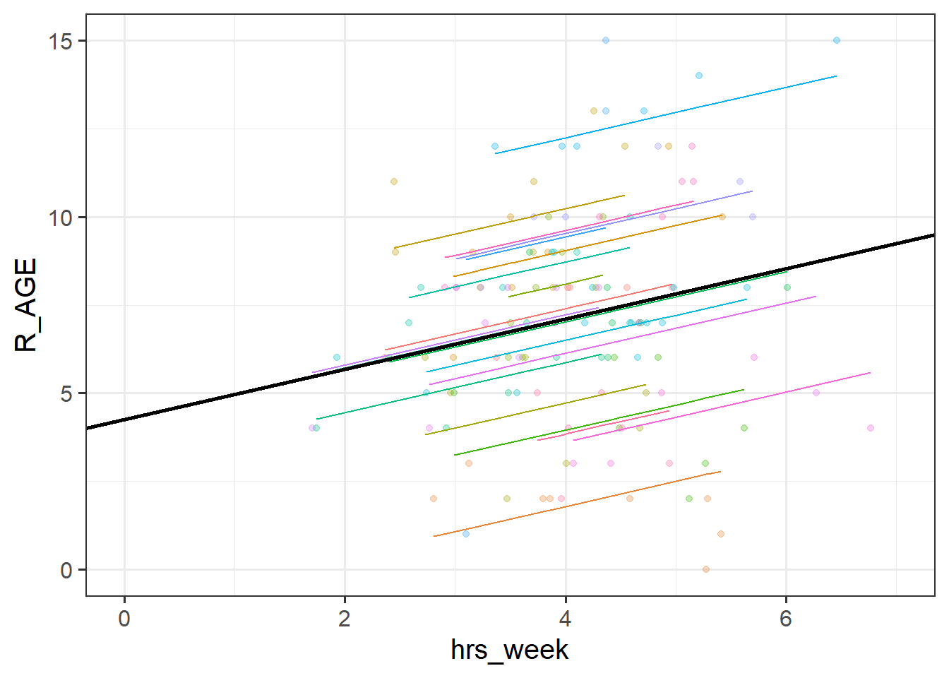
Match the parameters from the model equation, as well as coefficients from model output, to the corresponding points on the plot of fitted values.

Model Equation

• A1: \(\sigma_{0}\)
  
• A2: \(\sigma_{\varepsilon}\)
  
• A3: \(\gamma_{00}\)
  
• A4: \(b_{1}\)

Model Output

• B1: 0.7118
  
• B2: 2.698
  
• B3: 1.597
  
• B4: 4.2594

Plot of fitted values

• C1: the standard deviation of the distances from all the individual toy types lines to the black line
  
• C2: where the black line cuts the y axis
  
• C3: the slope of the black line
  
• C4: the standard deviation of the distances from all the individual observations to the line for the toy type to which it belongs.

• A1 = B2 = C1
• A2 = B3 = C4
• A3 = B4 = C2
• A4 = B1 = C3

Audio Interference in Executive Functioning

Data: Audio interference in executive functioning

This data is from a simulated study that aims to investigate the following research question:

How do different types of audio interfere with executive functioning, and does this interference differ depending upon whether or not noise-cancelling headphones are used?

30 healthy volunteers each completed the Symbol Digit Modalities Test (SDMT) - a commonly used test to assess processing speed and motor speed - a total of 15 times. During the tests, participants listened to either no audio (5 tests), white noise (5 tests) or classical music (5 tests). Half the participants listened via active-noise-cancelling headphones, and the other half listened via speakers in the room. Unfortunately, lots of the tests were not administered correctly, and so not every participant has the full 15 trials worth of data.

The data is available at https://uoepsy.github.io/data/efsdmt.csv.

variable	description
PID	Participant ID
audio	Audio heard during the test ('no_audio', 'white_noise','music')
headphones	Whether the participant listened via speakers in the room or via noise cancelling headphones
SDMT	Symbol Digit Modalities Test (SDMT) score

Question 8

How many participants are there in the data?
How many have complete data (15 trials)?
What is the average number of trials that participants completed? What is the minimum?
Does every participant have some data for each type of audio?

Hints

Functions like table() and count() will likely be useful here.

efdat <- read_csv("https://uoepsy.github.io/data/efsdmt.csv")
head(efdat)

# A tibble: 6 × 4
  PID    audio       headphones      SDMT
  <chr>  <chr>       <chr>          <dbl>
1 PPT_15 no_audio    speakers          37
2 PPT_22 no_audio    anc_headphones    55
3 PPT_21 no_audio    anc_headphones    40
4 PPT_20 no_audio    anc_headphones    36
5 PPT_20 no_audio    anc_headphones    30
6 PPT_05 white_noise speakers          30

For a quick “how many?”, functions like n_distinct() can be handy:

n_distinct(efdat$PID)

[1] 30

Which is essentially the same as asking:

unique(efdat$PID) |> length()

[1] 30

Here are the counts of trials for each participant.

efdat |> 
  count(PID)

# A tibble: 30 × 2
  PID        n
  <chr>  <int>
1 PPT_01    13
2 PPT_02    12
3 PPT_03    10
4 PPT_04    10
5 PPT_05    10
# ℹ 25 more rows

We can pass that to something like summary() to get a quick descriptive of the n column, and so we can see that no participant completed all 15 trials (max is 14). Everyone completed at least 10, and the median was 12.

efdat |> 
  count(PID) |>
  summary()

     PID                  n     
 Length:30          Min.   :10  
 Class :character   1st Qu.:11  
 Mode  :character   Median :12  
                    Mean   :12  
                    3rd Qu.:13  
                    Max.   :14  

We could also do this easily with things like:

table(efdat$PID) |> median()

[1] 12

For this kind of thing I would typically default to using table() for smaller datasets, to see how many datapoints are in each combination of PID and audio:

table(efdat$PID, efdat$audio)

        
         music no_audio white_noise
  PPT_01     4        5           4
  PPT_02     5        4           3
  PPT_03     3        2           5
  PPT_04     3        4           3
  PPT_05     5        2           3
  PPT_06     4        4           5
  PPT_07     4        3           4
  PPT_08     4        4           5
  PPT_09     5        4           5
  PPT_10     4        5           4
  PPT_11     4        4           4
  PPT_12     4        5           5
  PPT_13     4        4           3
  PPT_14     3        5           4
  PPT_15     4        5           4
  PPT_16     4        4           3
  PPT_17     5        4           5
  PPT_18     5        3           3
  PPT_19     3        5           3
  PPT_20     4        4           5
  PPT_21     3        5           4
  PPT_22     4        4           3
  PPT_23     3        3           4
  PPT_24     4        5           5
  PPT_25     4        4           5
  PPT_26     5        4           5
  PPT_27     5        2           4
  PPT_28     4        4           4
  PPT_29     4        4           4
  PPT_30     2        5           3

From the above, we can see that everyone has data from \(\geq 2\) trials for a given audio type.

table(efdat$PID, efdat$audio) |> min()

[1] 2

a tidyverse way:

When tables get too big, we can do the same thing with count(), but we need to make sure that we are working with factors, in order to summarise all possible combinations of groups (even empty ones)

efdat |> 
  mutate(PID = factor(PID),
         audio = factor(audio)) |>
  # the .drop=FALSE means "keep empty groups"
  count(PID,audio,.drop=FALSE) |> 
  summary()

      PID             audio          n    
 PPT_01 : 3   music      :30   Min.   :2  
 PPT_02 : 3   no_audio   :30   1st Qu.:4  
 PPT_03 : 3   white_noise:30   Median :4  
 PPT_04 : 3                    Mean   :4  
 PPT_05 : 3                    3rd Qu.:5  
 PPT_06 : 3                    Max.   :5  
 (Other):72                               

There are plenty of other ways (e.g., you could use combinations of group_by(), summarise()), so just pick one that makes sense to you.

Question 9

Consider the following questions about the study:

• What is our outcome of interest?
  
• What variables are we seeking to investigate in terms of their impact on the outcome?
  
• What are the units of observations?
  
• Are the observations clustered/grouped? In what way?
  
• What varies within these clusters?
  
• What varies between these clusters?

• What is our outcome of interest?
  • SDMT scores
    
• What variables are we seeking to investigate in terms of their impact on the outcome?
  • audio type and the interaction audio type \(\times\) wearing headphones
• What are the units of observations?
  • individual trials
    
• What are the groups/clusters?
  • participants
    
• What varies within these clusters?
  • the type of audio
    
• What varies between these clusters?
  • whether they listen via headphones or speakers

Question 10

Calculate the ICC, using the ICCbare() function from the ICC package.

How much of the variation in SDMT scores is attributable to participant level differences?

Hints

See 1A #icc, or look up the help documentation for ?ICCbare().

44% of the variance in SDMT scores is attributable to participant level differences.

library(ICC)
ICCbare(x = PID, y = SDMT, data = efdat)

[1] 0.4363587

Question 11

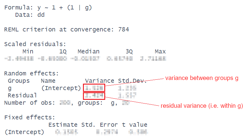
The multilevel model that has only an intercept (and the grouping structure) specified is sometimes referred to as the “null model” (or “intercept only model”).
Because there are no predictors in the fixed effects there is just a single value (the intercept). All of the variance in the outcome gets modelled in the random effects part, and is partitioned into either ‘variance between groups’ or ‘residual variance’. This means we can just use those estimates to calculate the ICC.

For our executive functioning study, fit the null model use the output to calculate the ICC.
Compare it to the answer from the previous question (it should be pretty close!)

Hints

The formula for the ICC is:
\[ ICC = \frac{\sigma^2_{b}}{\sigma^2_{b} + \sigma^2_e} = \frac{\text{between-group variance}}{\text{between-group variance}+\text{within-group variance}} \]

nullmod <- lmer(SDMT ~ 1 + (1 | PID), data = efdat)
summary(nullmod)

Linear mixed model fit by REML ['lmerMod']
Formula: SDMT ~ 1 + (1 | PID)
   Data: efdat

REML criterion at convergence: 2664.6

Scaled residuals: 
     Min       1Q   Median       3Q      Max 
-2.58680 -0.68262  0.03241  0.65701  2.26736 

Random effects:
 Groups   Name        Variance Std.Dev.
 PID      (Intercept) 62.02    7.875   
 Residual             79.82    8.934   
Number of obs: 360, groups:  PID, 30

Fixed effects:
            Estimate Std. Error t value
(Intercept)   34.789      1.514   22.98

\(\frac{62.02}{62.02+79.82} = 0.44\), or 44% of the variance in SDMT scores is explained by participant differences.

This matches (closely enough) with the ICCbare() function from the previous question!

Question 12

Make factors and set the reference levels of the audio and headphones variables to “no audio” and “speakers” respectively.

Hints

Can’t remember about setting factors and reference levels? Check back to USMR materials!

efdat <- efdat %>%
  mutate(
    audio = fct_relevel(factor(audio), "no_audio"),
    headphones = fct_relevel(factor(headphones), "speakers")
  )

Question 13

Fit a multilevel model to address the aims of the study (copied below)

How do different types of audio interfere with executive functioning, and does this interference differ depending upon whether or not noise-cancelling headphones are used?

Specifying the model may feel like a lot, but try splitting it into three parts:

\[ \text{lmer(}\overbrace{\text{outcome }\sim\text{ fixed effects}}^1\, + \, (1 + \underbrace{\text{slopes}}_3\, |\, \overbrace{\text{grouping structure}}^2 ) \]

1. Just like the lm()s we have used in USMR, think about what we want to test. This should provide the outcome and the structure of our fixed effects.
   
2. Think about how the observations are clustered/grouped. This should tell us how to specify the grouping structure in the random effects.
   
3. Think about which slopes (i.e. which terms in our fixed effects) could feasibly vary between the clusters. This provides you with what to put in as random slopes.

The question
    “How do different types of audio interfere with executive functioning” means we are interested in the effects of audio type (audio) on executive functioning (SDMT scores), so we will want:

lmer(SDMT ~ audio ...

However, the research aim also asks
    “… and does this interference differ depending upon whether or not noise-cancelling headphones are used?”
which suggests that we are interested in the interaction SDMT ~ audio * headphones

lmer(SDMT ~ audio * headphones + ...   

There are lots of ways that our data is grouped.
We have:

• 3 different groups of audio type (no_audio, white_noise, music)
• 2 groups of listening condition (speakers, anc_headphones)
• 30 groups of participants (“PPT_01”, “PPT_02”, “PPT_03”, …)

The effects of audio type and headphones are both things we actually want to test - these variables are in our fixed effects. The levels of audio and headphones are not just a random sample from a wider population of levels - they’re a specific set of things we want to compare SDMT scores between.

Compare this with the participants - we don’t care about if there is a difference in SDMT scores between e.g., “PPT_03” and “PPT_28”. The participants themselves are just a sample of people that we have taken from a wider population. This makes thinking of “by-participant random effects” a sensible approach - we model differences between participants as a normal distribution of deviations around some average:

lmer(SDMT ~ audio * headphones + (1 + ... | PID)  

The minimum that we can include is the random intercept. What (1|PID) specifies is that “participants vary in their SDMT scores”. This makes sense - we would expect some participants to have higher executive functioning (and so will tend to score high on the SDMT), and others to have lower functioning (and so tend to score lower).

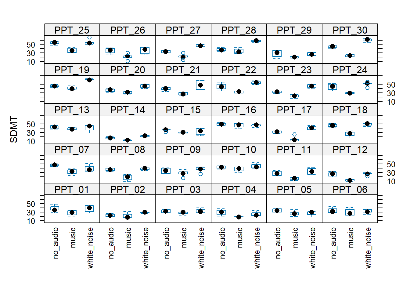
We can also include a random by-participant effect of audio.
audio|PID specifies that the effect of audio type on SDMT varies by participant. This seems feasible - music might be very distracting (and interfere a lot with the test) for some participants, but have a negligible effect for others.

lmer(SDMT ~ audio * headphones + 
              (1 + audio | PID), data = efdat)

Why can’t we have (headphones|PID)?

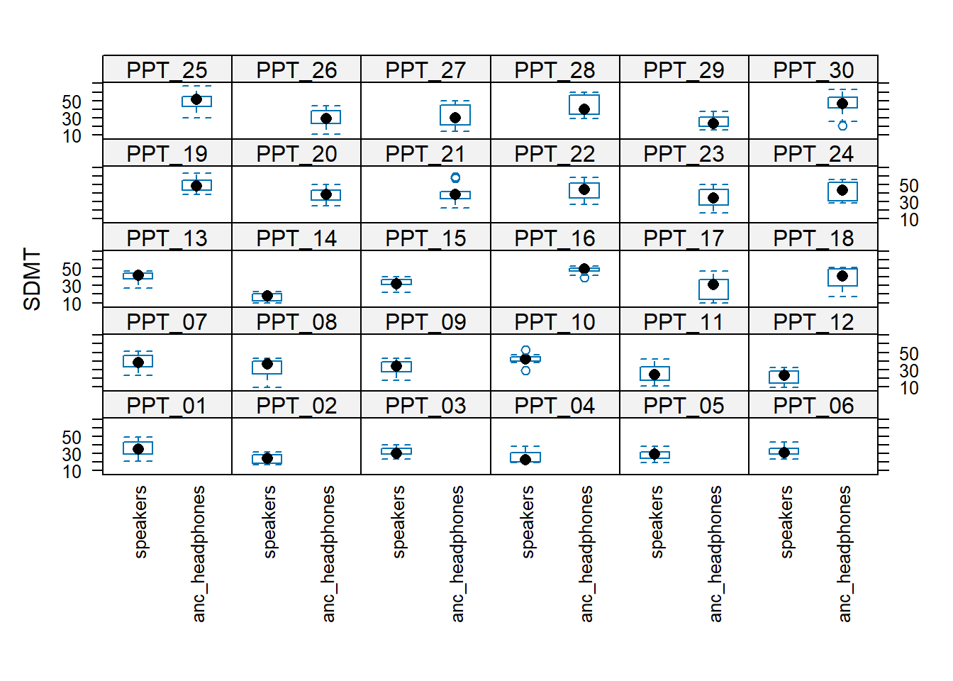
Why can we fit (1 + audio | PID) but not (1 + headphones | PID), or both (1 + audio + headphones | PID) or (1 + audio * headphones | PID)?

Remember that y ~ ... + (x | g) is saying “the slope of y~x varies by g”.
Such a sentence only makes sense if each “the slope of y~x” is defined for every (or most) groups.

For the headphones predictor, every participant is either in the “speakers” condition or the “anc_headphones” condition.
This means that “the effect of headphones on SDMT” doesn’t exist for any single participant! This means it makes no sense to try and think of the effect as ‘varying by participant’.

Compare this to the audio predictor, for the effect does exist for a single given participant, therefore it is possible to think of it as being different for different participants (e.g. PPT_30’s performance improves with white noise, but PPT_16’s performance does not).

The plots below may help to cement this idea:

Question 14

We now have a model, but we don’t have any p-values or confidence intervals or anything - i.e. we have no inferential criteria on which to draw conclusions. There are a whole load of different methods available for drawing inferences from multilevel models, which means it can be a bit of a never-ending rabbit hole. For now, we’ll just use the ‘quick and easy’ approach provided by the lmerTest package seen in the lectures.

Using the lmerTest package, re-fit your model, and you should now get some p-values!

Hints

If you use library(lmerTest) to load the package, then every single model you fit will show p-values calculated with the Satterthwaite method.
Personally, I would rather this is not the case, so I often opt to fit specific models with these p-values without ever loading the package:
modp <- lmerTest::lmer(y ~ 1 + x + ....

optional: a model comparison

If we want to go down the model comparison route, we just need to isolate the relevant part(s) of the model that we are interested in.

Remember, as we saw in USMR, model comparison is sometimes a useful way of testing a set of coefficients. For instance, in this example the interaction involves estimating two terms: audiomusic:headphonesanc_headphones and audiowhite_noise:headphonesanc_headphones.

To test the interaction as a whole, we can create a model without the interaction, and then compare it. The SATmodcomp() function from the pbkrtest package provides a way of conducting an F test with the same Satterthwaite method of approximating the degrees of freedom:

sdmt_mod <- lmer(SDMT ~ audio * headphones + 
              (1 + audio | PID), data = efdat)
sdmt_res <- lmer(SDMT ~ audio + headphones + 
                   (1 + audio | PID), data = efdat)
library(pbkrtest)
SATmodcomp(largeModel = sdmt_mod, smallModel = sdmt_res)

large : SDMT ~ audio * headphones + (1 + audio | PID)
small (restriction matrix) : 
                             
 0 0 0 0 0.8936904 -0.4486841
 0 0 0 0 0.4486841  0.8936904
     statistic    ndf    ddf   p.value    
[1,]    11.051  2.000 26.909 0.0003136 ***
---
Signif. codes:  0 '***' 0.001 '**' 0.01 '*' 0.05 '.' 0.1 ' ' 1

sdmt_mod <- lmerTest::lmer(SDMT ~ audio * headphones + 
              (1 + audio | PID), data = efdat)

summary(sdmt_mod)

Linear mixed model fit by REML. t-tests use Satterthwaite's method [
lmerModLmerTest]
Formula: SDMT ~ audio * headphones + (1 + audio | PID)
   Data: efdat

REML criterion at convergence: 2376.2

Scaled residuals: 
     Min       1Q   Median       3Q      Max 
-2.34520 -0.62861  0.05762  0.60807  2.21250 

Random effects:
 Groups   Name             Variance Std.Dev. Corr       
 PID      (Intercept)      51.17    7.153               
          audiomusic       13.69    3.700     0.03      
          audiowhite_noise 15.22    3.901    -0.25 -0.16
 Residual                  31.49    5.612               
Number of obs: 360, groups:  PID, 30

Fixed effects:
                                          Estimate Std. Error       df t value
(Intercept)                               33.25799    1.98897 28.22064  16.721
audiomusic                                -8.01731    1.41149 27.58766  -5.680
audiowhite_noise                          -0.03044    1.44502 26.32588  -0.021
headphonesanc_headphones                   6.85313    2.81170 28.19226   2.437
audiomusic:headphonesanc_headphones       -3.58748    2.00129 27.94011  -1.793
audiowhite_noise:headphonesanc_headphones  8.02458    2.04498 26.46166   3.924
                                          Pr(>|t|)    
(Intercept)                               3.54e-16 ***
audiomusic                                4.58e-06 ***
audiowhite_noise                          0.983354    
headphonesanc_headphones                  0.021355 *  
audiomusic:headphonesanc_headphones       0.083875 .  
audiowhite_noise:headphonesanc_headphones 0.000556 ***
---
Signif. codes:  0 '***' 0.001 '**' 0.01 '*' 0.05 '.' 0.1 ' ' 1

Correlation of Fixed Effects:
            (Intr) audmsc adwht_ hdphn_ adms:_
audiomusic  -0.174                            
audiowht_ns -0.352  0.192                     
hdphnsnc_hd -0.707  0.123  0.249              
admsc:hdph_  0.123 -0.705 -0.135 -0.173       
adwht_ns:h_  0.249 -0.136 -0.707 -0.351  0.191

Question 15

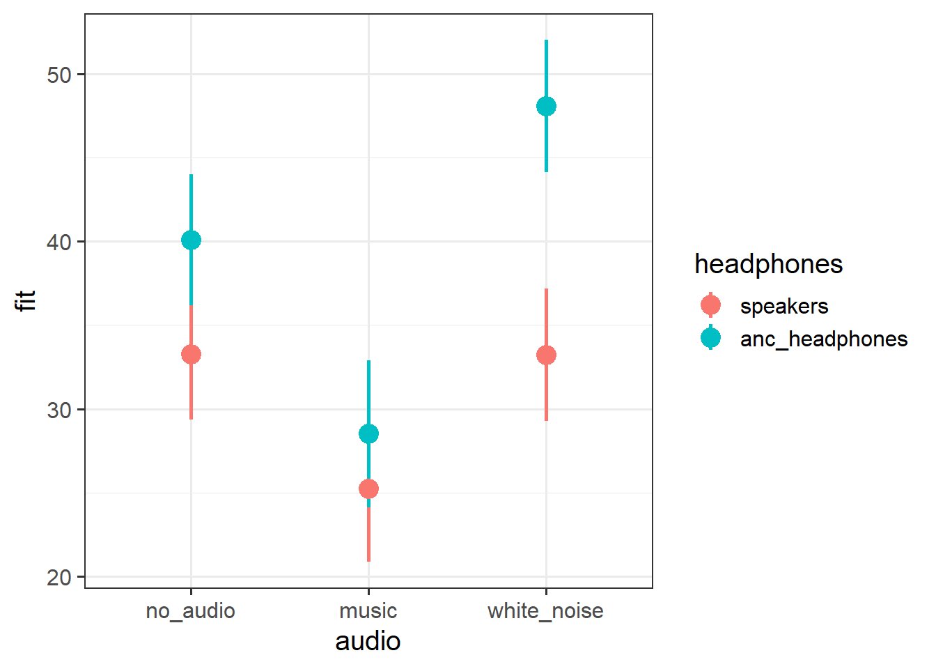
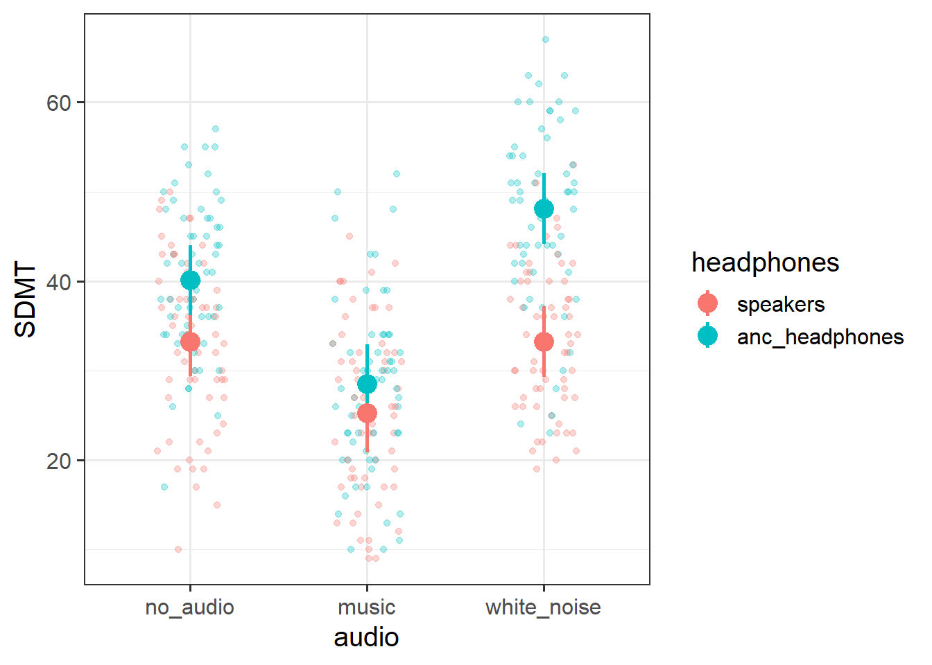
We’ve already seen in the example with the toys (above) that we can visualise the fitted values (model predictions) using things like augment() from the broom.mixed package. But these were plotting all the cluster-specific values (i.e. our random effects), and what we are really interested in are the estimates of (and uncertainty around) our fixed effects.

Using tools like the effects package can provide us with the values of the outcome across levels of a specific fixed predictor (holding other predictors at their mean).

library(effects)
effect(term = "audio*headphones", mod = sdmt_mod) |>
  as.data.frame() |>
  ggplot(aes(x=audio,y=fit,
             ymin=lower,ymax=upper,
             col=headphones))+
  geom_pointrange(size=1,lwd=1)

Question 16

Now we have some p-values and a plot, try to create a short write-up of the analysis and results.

SDMT scores were modelled using linear mixed effects regression, with fixed effects of audio-type (no audio/white noise/music, treatment coded with no audio as the reference level), audio delivery (speakers/ANC-headphones, treatment coded with speakers as the reference level) and their interaction. Participant-level random intercepts and random slopes of audio-type were also included. The model was fitted using the lme4 package in R, and estimated with restricted estimation maximum likelihood (REML). Denominator degrees of freedom for all tests were approximated using the Satterthwaite method.

Inclusion of the interaction between headphones and audio-type was found to improve model fit (\(F(2, 26.9) = 11.05, p < .001\)), suggesting that the interference of different types of audio on executive functioning is dependent upon whether the audio is presented through ANC-headphones or through speakers.
Participants not wearing headphones and presented with no audio scored on average 33.26 on the SDMT. Listening to music via speakers was associated with lower scores (\(b = -8.02, t(27.59)=-5.68, p <0.001\)) compared to no audio. White noise played via speakers was not associated with a difference in performance on the SDMT compared to no audio.

Without any audio playing, wearing ANC-headphones was associated with higher SDMT scores compared to no headphones (\(b = 6.85, t(28.19)=2.44, p =0.021\)). This difference between headphones and speakers was also evident when listening to white-noise (\(b = 8.02, t(26.46)=3.92, p <0.001\)). The apparent detrimental influence of music was not found to differ depending on whether headphones were worn (\(b = -3.59, p =0.084\)).

These results suggest that while music appears to interfere with executive functioning (resulting in lower SDMT scores) regardless of whether it is heard through headphones or speakers, listening to white noise may actually improve executive functioning, but only when presented via headphones. Furthermore, there appears to be benefits for executive functioning from wearing ANC-headphones even when not-listening to audio, perhaps due to the noise cancellation. The pattern of findings are displayed in Figure 1.

Figure 1: Interaction between the type (no audio/white noise/music) and the delivery (speakers/ANC headphones) on executive functioning task (SDMT)

Footnotes

1. Image sources:
   http://tophatsasquatch.com/2012-tmnt-classics-action-figures/
   https://www.dezeen.com/2016/02/01/barbie-dolls-fashionista-collection-mattel-new-body-types/
   https://www.wish.com/product/5da9bc544ab36314cfa7f70c
   https://www.worldwideshoppingmall.co.uk/toys/jumbo-farm-animals.asp
   https://www.overstock.com/Sports-Toys/NJ-Croce-Scooby-Doo-5pc.-Bendable-Figure-Set-with-Scooby-Doo-Shaggy-Daphne-Velma-and-Fred/28534567/product.html
   https://tvtropes.org/pmwiki/pmwiki.php/Toys/Furby
   https://www.fun.com/toy-story-4-figure-4-pack.html
   https://www.johnlewis.com/lego-minifigures-71027-series-20-pack/p5079461