Week 2 Exercises: Logistic and Longitudinal

Great Apes!

Data: msmr_apespecies.csv & msmr_apeage.csv

We have data from a large sample of great apes who have been studied between the ages of 1 to 10 years old (i.e. during adolescence). Our data includes 4 species of great apes: Chimpanzees, Bonobos, Gorillas and Orangutans. Each ape has been assessed on a primate dominance scale at various ages. Data collection was not very rigorous, so apes do not have consistent assessment schedules (i.e., one may have been assessed at ages 1, 3 and 6, whereas another at ages 2 and 8).

The researchers are interested in examining how the adolescent development of dominance in great apes differs between species.

Data on the dominance scores of the apes are available at https://uoepsy.github.io/data/msmr_apeage.csv and the information about which species each ape is are in https://uoepsy.github.io/data/msmr_apespecies.csv.

Table 1:

Data Dictionary: msmr_apespecies.csv

variable	description
ape	Ape Name
species	Species (Bonobo, Chimpanzee, Gorilla, Orangutan)

Table 2:

Data Dictionary: msmr_apeage.csv

variable	description
ape	Ape Name
age	Age at assessment (years)
dominance	Dominance (Z-scored)

Question 1

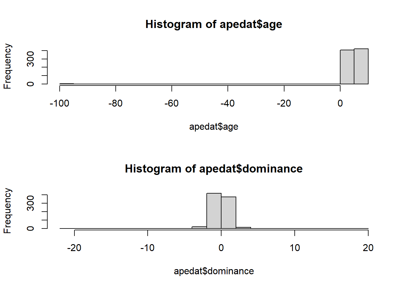
Read in the data and check over it. Do any relevant cleaning/wrangling that might be necessary.

We’ll read in both datasets, and then join them together.

library(tidyverse)
library(lme4)
ape_species <- read_csv("https://uoepsy.github.io/data/msmr_apespecies.csv")
ape_age <- read_csv("https://uoepsy.github.io/data/msmr_apeage.csv")

Sometimes is handy to check that all our participants are in both datasets:

# are all the apes in ape_age also in ape_species?
all(ape_age$ape %in% ape_species$ape)

[1] TRUE

# and vice versa?
all(ape_species$ape %in% ape_age$ape)

[1] TRUE

Let’s join them:

apedat <- full_join(ape_age, ape_species)
head(apedat)

# A tibble: 6 × 4
  ape     age dominance species   
  <chr> <dbl>     <dbl> <chr>     
1 Joel      7       0.6 chimpanzee
2 Joel      5       1.2 chimpanzee
3 Joel      8       1.1 chimpanzee
4 Joel      1       0.2 chimpanzee
5 Joel      2       0.5 chimpanzee
6 Joel      6       1   chimpanzee

First off, we can see that we’ve got some weird typos. Some apes have been identified as “gorrila” but it is actually spelled “gorilla”.
Also, we’ve got people using two alternatives for the chimps: “chimp” and “chimpanzee”. We’ll need to combine those.

table(apedat$species)

    bonobo      chimp chimpanzee    gorilla    gorrila  orangutan 
       187        146        127        211          2        157 

Age looks like it has some weird values (possibly “-99”?), and there are possibly a few outliers in the dominance variable. Given that dominance is standardised, it is extremely unlikely that we would see values around 20.. They’re not “impossible”, but they’re so incredibly unlikely that I’d be more comfortable assuming they are typos:

hist(apedat$age, breaks=20)
hist(apedat$dominance, breaks=20)

Just to see what the most extreme values of dominance are:

# show the biggest 5 absolute values in dominance variable
sort(abs(apedat$dominance), decreasing = TRUE)[1:5]

[1] 21.2 19.4  3.9  2.9  2.9

apedat <- apedat |> 
  mutate(
    # fix species typos
    species = case_when(
      species %in% c("chimp","chimpanzee") ~ "chimp",
      species %in% c("gorilla","gorrila") ~ "gorilla",
      TRUE ~ species
    )
  ) |>
    filter(
      # get rid of ages -99
      age > 0, 
      # keep when dominance is between -5 and 5 
      # (5 here is a slightly arbitrary choice, but you can see from
      # our checks that this will only exclude the two extreme datapoints
      # that are 21.2 and 19.4
      (dominance < 5 & dominance > -5) 
    )

Question 2

How is this data structure “hierarchical” (or “clustered”)? What are our level 1 units, and what are our level 2 units?

We have a random sample of \(\underbrace{\text{timepoints}}_{\text{level 1}}\) from a random sample of \(\underbrace{\text{apes}}_{\text{level 2}}\).

Question 3

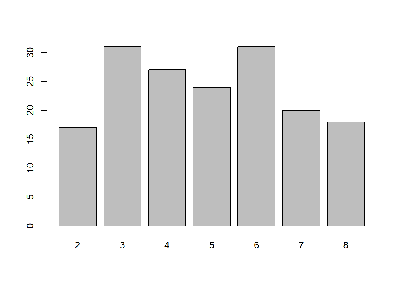
For how many apes do we have data? How many of each species?
How many datapoints does each ape have?

Hints

We’ve seen this last week too - counting the different levels in our data. See 2B #getting-to-know-my-monkeys for an example (with another monkey example!)

We have 168 apes in our dataset:

length(unique(apedat$ape))

[1] 168

Here’s how many of each species:

apedat |> 
  group_by(species) |>
  summarise(
   n_apes = n_distinct(ape) 
  )

# A tibble: 4 × 2
  species   n_apes
  <chr>      <int>
1 bonobo        36
2 chimp         56
3 gorilla       46
4 orangutan     30

Let’s create a table of how many observations for each ape, and then we can create a table from that table, to show how many apes have 2 datapoints, how many have 3, 4, and so on:

table(apedat$ape) |>
  table() |>
  barplot()

Question 4

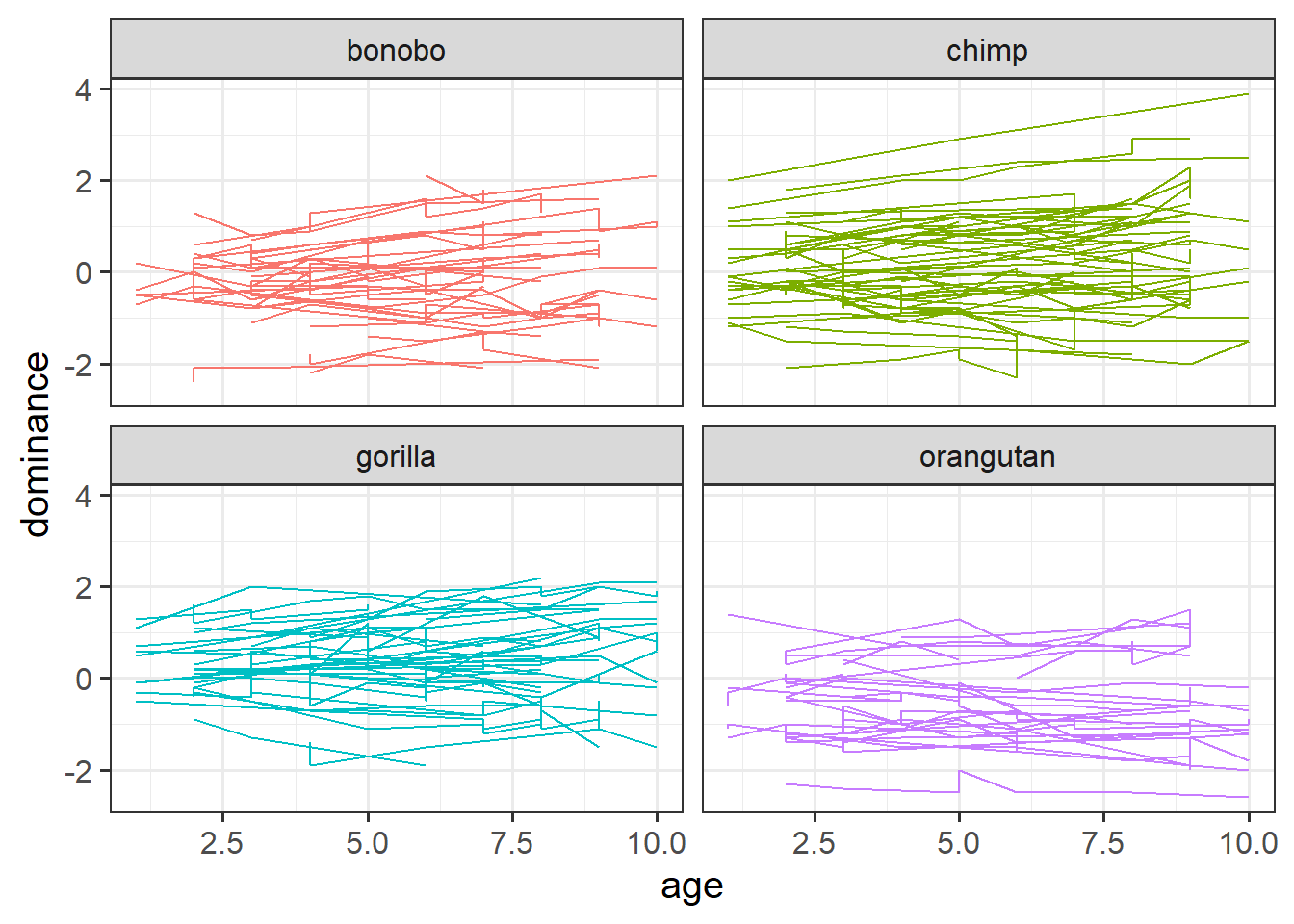
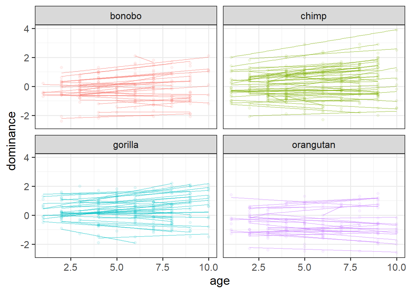
Make a plot to show how dominance changes as apes get older.

Hints

In 2B #exploring-the-data we made a facet for each cluster (each participant). That was fine because we had only 20 people. In this dataset we have 168! That’s too many to facet. The group aesthetic will probably help instead!

Here’s a line for each ape, and a facet for each species:

ggplot(apedat, aes(x = age, y = dominance, col = species))+
  geom_line(aes(group = ape)) + 
  facet_wrap(~species) + 
  guides(col="none")

It’s kind of hard to see the trend for each ape, so let’s also make a separate little linear model for each ape:

ggplot(apedat, aes(x = age, y = dominance, col = species))+
  geom_point(alpha=.1) +
  stat_smooth(aes(group=ape),geom="line",method=lm,se=F,alpha=.5) +
  facet_wrap(~species) + 
  guides(col="none")

Question 5

Recenter the age variable on 1, which is the youngest ages that we’ve got data on for any of our species.

Then fit a model that estimates the differences between primate species in how dominance changes over time.

apedat$age = apedat$age-1 

m.full <- lmer(dominance ~ 1 + age * species + (1 + age | ape), data = apedat)

Question 6

Do primate species differ in the growth of dominance?
Perform an appropriate test/comparison.

Hints

This is asking about the age*species interaction, which in our model is represented by 3 parameters. To assess the overall question, it might make more sense to do a model comparison.

m.int <- lmer(dominance ~ 1 + age + species + (1 + age | ape), data = apedat)

anova(m.int, m.full)

Data: apedat
Models:
m.int: dominance ~ 1 + age + species + (1 + age | ape)
m.full: dominance ~ 1 + age * species + (1 + age | ape)
       npar    AIC    BIC  logLik deviance  Chisq Df Pr(>Chisq)   
m.int     9 806.67 849.11 -394.34   788.67                        
m.full   12 801.16 857.74 -388.58   777.16 11.517  3   0.009237 **
---
Signif. codes:  0 '***' 0.001 '**' 0.01 '*' 0.05 '.' 0.1 ' ' 1

Species differ in how dominance changes over adolescence (\(\chi^2(3) = 11.52, p = 0.009\)).

Question 7

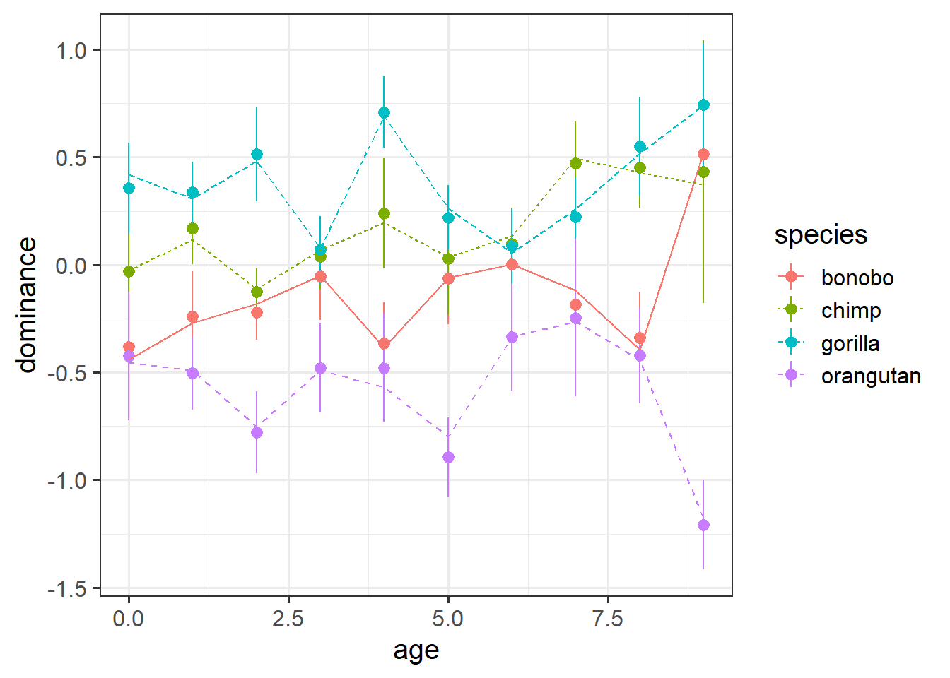
Plot the average model predicted values for each age.

Before you plot.. do you expect to see straight lines? (remember, not every ape is measured at age 2, or age 3, etc).

Hints

This is like taking predict() from the model, and then then grouping by age, and calculating the mean of those predictions. However, we can do this more easily using augment() and then some fancy stat_summary() in ggplot (see the lecture).

Averaging fitted values would give us straight lines if every ape had data at all ages, but in our study we have some apes with only 2 data points, and each ape has different set of ages (e.g., one ape might be measured at age 3, 6, and 10, another ape might be at ages 2 and 16).

library(broom.mixed)

augment(m.full) |>
ggplot(aes(age,dominance, color=species)) +
  # the point ranges are our observations
  stat_summary(fun.data=mean_se, geom="pointrange") + 
  # the lines are our average predictions  
  stat_summary(aes(y=.fitted, linetype=species), fun=mean, geom="line")

Question 8

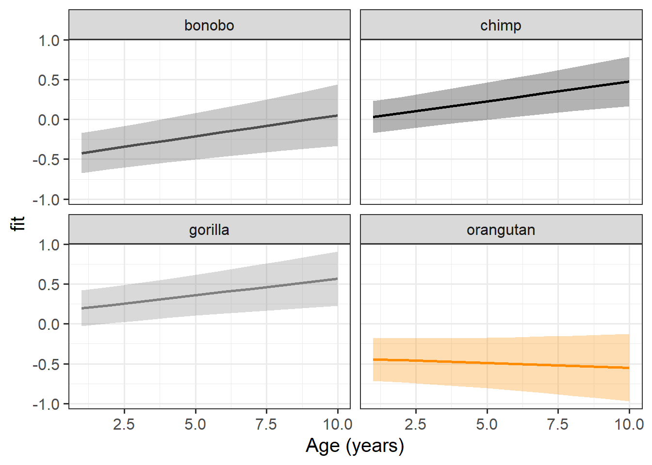
Plot the model based fixed effects:

effects::effect("age*species", m.full, xlevels=10) |>
  as.data.frame() |>
  ggplot(aes(x=age+1,y=fit,col=species))+
  geom_line(lwd=1)+
  geom_ribbon(aes(ymin=lower,ymax=upper,fill=species),col=NA,alpha=.3) +  
  scale_color_manual(values=c("grey30","black","grey50","darkorange")) +
  scale_fill_manual(values=c("grey30","black","grey50","darkorange")) +
  facet_wrap(~species) + 
  guides(col="none",fill="none") +
  labs(x="Age (years)")

Question 9

Interpret each of the fixed effects from the model (you might also want to get some p-values or confidence intervals).

Hints

Each of the estimates should correspond to part of our plot from the previous question.

Let’s get some confidence intervals:

confint(m.full, method="profile",
        parm = "beta_")

                           2.5 %      97.5 %
(Intercept)          -0.67066925 -0.17299177
age                   0.02361398  0.08142209
specieschimp          0.13383485  0.77009884
speciesgorilla        0.28124162  0.94933844
speciesorangutan     -0.38909919  0.34257548
age:specieschimp     -0.03973125  0.03392308
age:speciesgorilla   -0.05012759  0.02799394
age:speciesorangutan -0.10625760 -0.02167806

term	est	CI	interpretation
(Intercept)	-0.42	[-0.67, -0.17]*	estimated dominance of 1 year old bonobos (at left hand side of plot, bonobo line is lower than 0)
age	0.05	[0.02, 0.08]*	estimated change in dominance score for every year older a bonobo gets (slope of bonobo line)
specieschimp	0.45	[0.13, 0.77]*	estimated difference in dominance scores at age 1 between bonobos and chimps (at left hand side of plot, chimp line is higher than bonobo line)
speciesgorilla	0.62	[0.28, 0.95]*	estimated difference in dominance scores at age 1 between bonobos and gorillas (at left hand side of plot, gorilla line is higher than bonobo line)
speciesorangutan	-0.02	[-0.39, 0.34]	no significant difference in dominance scores at age 1 between bonobos and orangutans (at the left hand side of our plot, orangutan line is similar height to bonobo line)
age:specieschimp	0.00	[-0.04, 0.03]	no significant difference between chimps and bonobos in the change in dominance for every year older (slope of chimp line is similar to slope of bonobo line)
age:speciesgorilla	-0.01	[-0.05, 0.03]	no significant difference between gorillas and bonobos in the change in dominance for every year older (slope of gorilla line is similar to slope of bonobo line)
age:speciesorangutan	-0.06	[-0.11, -0.02]*	estimated difference between orangutans and bonobos in the change in dominance for every year older (slope of orangutan line is less steep than slope of bonobo line)

Trolley problems

Data: msmr_trolley.csv

The “Trolley Problem” is a thought experiment in moral philosophy that asks you to decide whether or not to pull a lever to divert a trolley. Pulling the lever changes the trolley direction from hitting 5 people to a track on which it will hit one person.

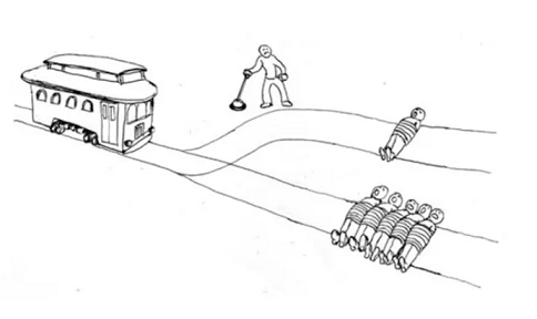
Previous research has found that the “framing” of the problem will influence the decisions people make:

positive frame	neutral frame	negative frame
5 people will be saved if you pull the lever; one person on another track will be saved if you do not pull the lever. All your actions are legal and understandable. Will you pull the lever?	5 people will be saved if you pull the lever, but another person will die. One people will be saved if you do not pull the lever, but 5 people will die. All your actions are legal and understandable. Will you pull the lever?	One person will die if you pull the lever. 5 people will die if you do not pull the lever. All your actions are legal and understandable. Will you pull the lever?

We conducted a study to investigate whether the framing effects on moral judgements depends upon the stakes (i.e. the number of lives saved).

120 participants were recruited, and each gave answers to 12 versions of the thought experiment. For each participant, four versions followed each of the positive/neutral/negative framings described above, and for each framing, 2 would save 5 people and 2 would save 15 people.

The data are available at https://uoepsy.github.io/data/msmr_trolley.csv.

Table 3:

Data Dictionary: trolley.csv

variable	description
PID	Participant ID
frame	framing of the thought experiment (positive/neutral/negative
lives	lives at stake in the thought experiment (5 or 15)
lever	Whether or not the participant chose to pull the lever (1 = yes, 0 = no)

Question 10

Read in the data and check over how many people we have, and whether we have complete data for each participant.

Hints

I would maybe try data |> group_by(participant) |> summarise(), and then use the n_distinct() function to count how many “things” each person sees (e.g., 2B #example).

trolley <- read_csv("https://uoepsy.github.io/data/msmr_trolley.csv")
head(trolley)

# A tibble: 6 × 4
  PID   frame    lives   lever
  <chr> <chr>    <chr>   <dbl>
1 PPT_1 positive 5lives      1
2 PPT_1 positive 15lives     1
3 PPT_1 positive 5lives      1
4 PPT_1 positive 15lives     1
5 PPT_1 neutral  5lives      1
6 PPT_1 neutral  15lives     0

How many participants?

length(unique(trolley$PID))

[1] 120

How many trials for each participant in each condition.
We can, for each participant, count how many trials they have in total, how many “frames” they see, how many “lives” they see, and how many “frame x lives” combinations they see:

trolley |>
  group_by(PID) |>
  summarise(
    n_trials = n(),
    n_frame = n_distinct(frame),
    n_lives = n_distinct(lives),
    n_combn = n_distinct(frame,lives)
  )

# A tibble: 120 × 5
   PID     n_trials n_frame n_lives n_combn
   <chr>      <int>   <int>   <int>   <int>
 1 PPT_1         12       3       2       6
 2 PPT_10        12       3       2       6
 3 PPT_100       12       3       2       6
 4 PPT_101       12       3       2       6
 5 PPT_102       12       3       2       6
 6 PPT_103       12       3       2       6
 7 PPT_104       12       3       2       6
 8 PPT_105       12       3       2       6
 9 PPT_106       12       3       2       6
10 PPT_107       12       3       2       6
# ℹ 110 more rows

If everybody gets the same here (as we can see they do below), then everyone has complete data!

trolley |>
  group_by(PID) |>
  summarise(
    n_trials = n(),
    n_frame = n_distinct(frame),
    n_lives = n_distinct(lives),
    n_combn = n_distinct(frame,lives)
  ) |>
  summary()

     PID               n_trials     n_frame     n_lives     n_combn 
 Length:120         Min.   :12   Min.   :3   Min.   :2   Min.   :6  
 Class :character   1st Qu.:12   1st Qu.:3   1st Qu.:2   1st Qu.:6  
 Mode  :character   Median :12   Median :3   Median :2   Median :6  
                    Mean   :12   Mean   :3   Mean   :2   Mean   :6  
                    3rd Qu.:12   3rd Qu.:3   3rd Qu.:2   3rd Qu.:6  
                    Max.   :12   Max.   :3   Max.   :2   Max.   :6  

Question 11

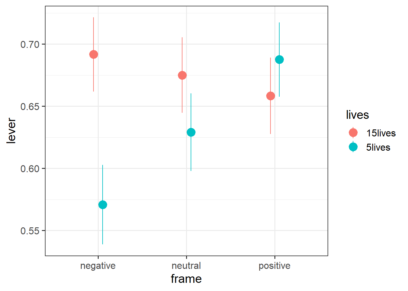
Construct an appropriate plot to summarise the data in a suitable way to illustrate the research question.

Hints

Something making use of stat_summary() to give proportions, a bit like the plot in 2B #getting-to-know-my-monkeys?

Here is a plot of proportions of trials in which the lever was pulled, split by how the problem was framed, and the number of lives saved:

ggplot(trolley, aes(x=frame, y=lever, col=lives)) +
  stat_summary(geom="pointrange", size=1, 
               position=position_dodge(width=.2)) 

Question 12

Fit a model to assess the research aims.
Don’t worry if it gives you an error, we’ll deal with that in a second.

Hints

• Remember, a good way to start is to split this up into 3 parts: 1) the outcome and fixed effects, 2) the grouping structure, and 3) the random slopes.
  
• fitting (or attempting to fit!) glmer models might take time!

The researchers are “interested in whether the framing effects on moral judgements depends upon the stakes (i.e. the number of lives saved)”.

“the framing effect on moral judgements” here is operationalised as

lever ~ frame

and the wording “depends upon the stakes” means that we want to know if that effect of frame “is different for” the situations when lives = 5, vs lives = 15 - i.e. we need the interaction!

lever ~ frame * lives

The outcome here is lever pulled (yes v no), so it’s a binary variable!

glmer(lever ~ frame * lives + ....
      ....,  
      data = trolley, family = binomial)

We know that we have multiple observations for each participant, and those participants are just a random sample (it’s not something we’re interested in testing, we would like to model participant differences as random variation).

glmer(lever ~ frame * lives + ....
      (1 + .... | PID),  
      data = trolley, family = binomial)

Finally, what effects could theoretically vary between our participants?
Every participant saw everything (i.e. both frame and lives are “within participant” variables).

In theory, all of these are possible given our design:

• the effect of frame on probability of pulling the lever could vary between participants
• the effect of number of lives on probability of pulling the lever could vary between participants
• the amount by which number of lives influences the effect of frame on pulling the lever could vary between participants

So we could theoretically try and fit this model:

mod1 <- glmer(lever ~ frame * lives + 
      (1 + frame * lives | PID),  
      data = trolley, family = binomial)

Warning messages:
1: In (function (fn, par, lower = rep.int(-Inf, n), upper = rep.int(Inf, : failure to converge in 10000 evaluations
2: In optwrap(optimizer, devfun, start, rho$lower, control = control, : convergence code 4 from Nelder_Mead: failure to converge in 10000 evaluations
3: In checkConv(attr(opt, “derivs”), opt$par, ctrl = control$checkConv, : Model failed to converge with max|grad| = 0.0795145 (tol = 0.002, component 1)

Question 13

This is probably the first time we’ve had to deal with a model not converging.

While sometimes changing the optimizer can help, more often than not, the model we are trying to fit is just too complex. Often, the groups in our sample just don’t vary enough for us to estimate a random slope.

The aim here is to simplify our random effect structure in order to obtain a converging model, but be careful not to over simplify.

Try it now. What model do you end up with? (You might not end up with the same model as each other, which is fine. These methods don’t have “cookbook recipes”!)

Hints

you could think of the interaction as the ‘most complex’ part of our random effects, so you might want to remove that first.

This model still does not converge:

mod2 <- glmer(lever ~ frame * lives + 
      (1 + frame + lives | PID),  
      data = trolley, family = binomial)

Warning message:
In checkConv(attr(opt, “derivs”), opt$par, ctrl = control$checkConv, : Model failed to converge with max|grad| = 0.00734804 (tol = 0.002, component 1)

We have a choice here - do we remove frame|PID or lives|PID? One practical point is that each participant has only 4 observations for each frame type, but they have 6 observations for each lives type, which might make it easier to fit.

mod3 <- glmer(lever ~ frame * lives + 
      (1 + lives | PID),  
      data = trolley, family = binomial)

Hooray! it converges!

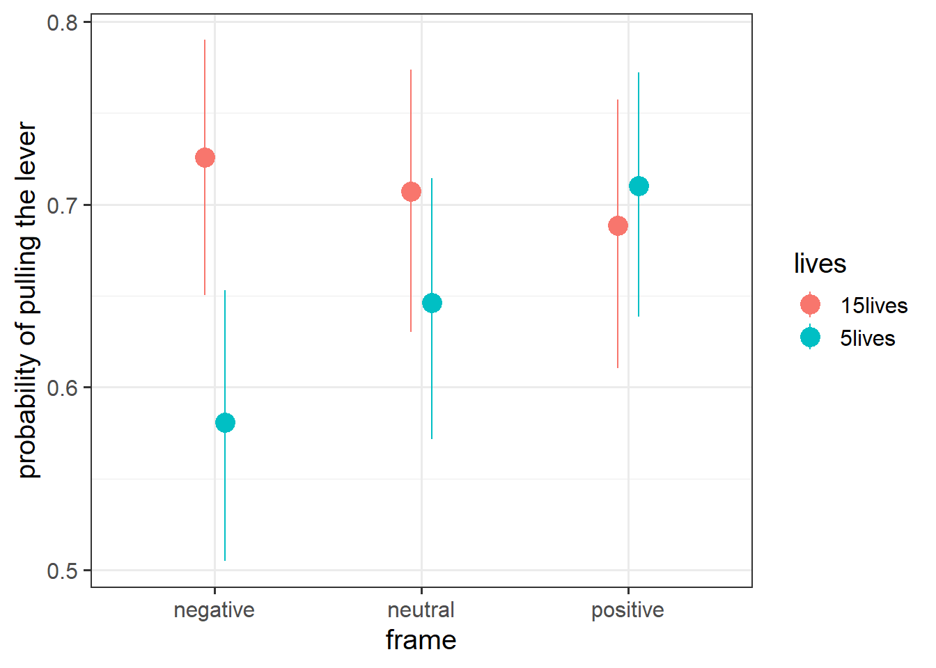
Question 14

Plot the predicted probabilities from your model for each combination of frame and lives.

library(effects)
effect("frame*lives", mod3) |>
  as.data.frame() |>
  ggplot(aes(x = frame, y = fit, col = lives)) +
  geom_pointrange(aes(ymin=lower,ymax=upper),
                  position=position_dodge(width=.2),
                  size=1)+
  labs(y="probability of pulling the lever")

Optional extra: Novel Word Learning

Data: nwl.Rdata

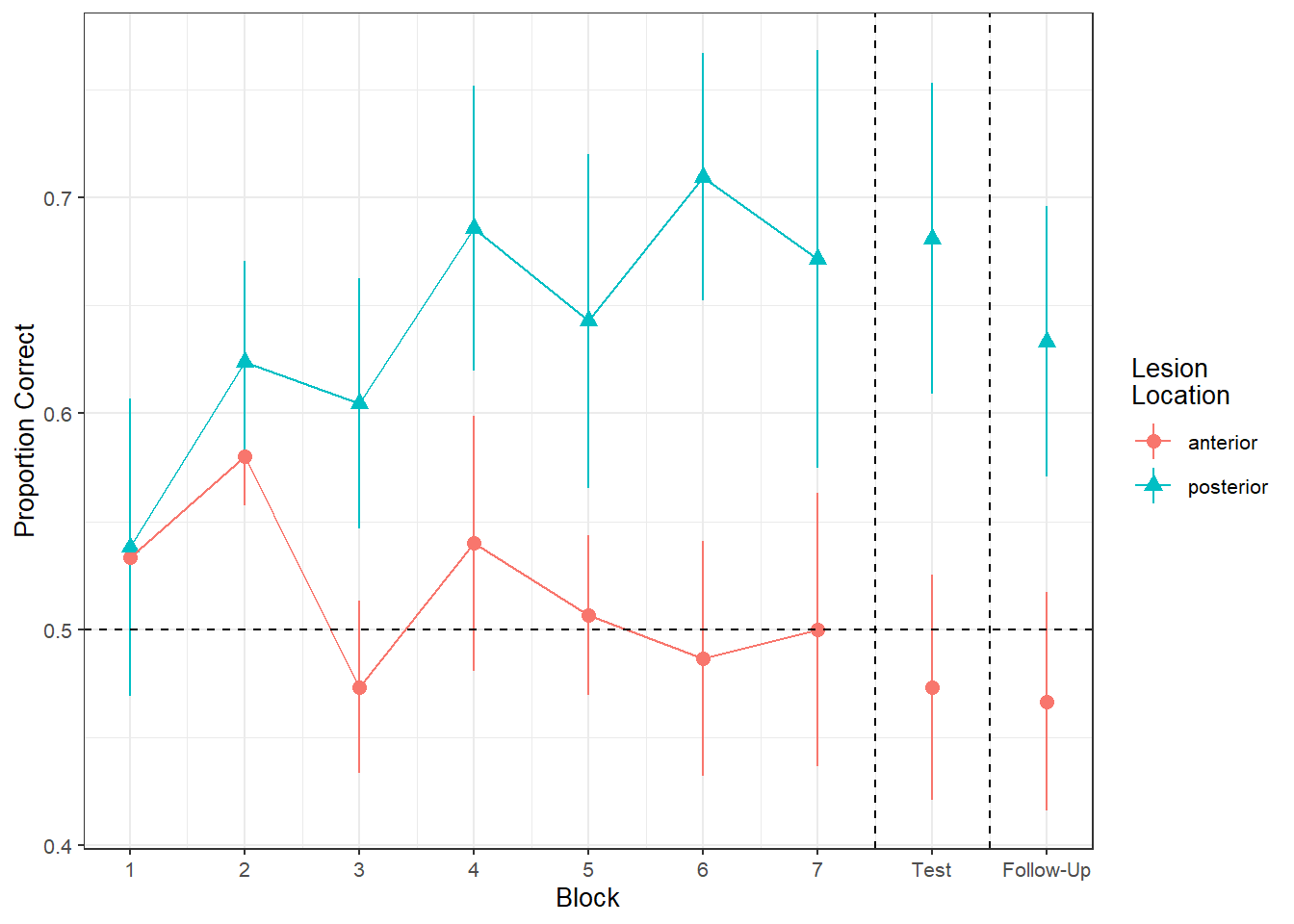
load(url("https://uoepsy.github.io/msmr/data/nwl.RData"))

In the nwl data set (accessed using the code above), participants with aphasia are separated into two groups based on the general location of their brain lesion: anterior vs. posterior. There is data on the numbers of correct and incorrect responses participants gave in each of a series of experimental blocks. There were 7 learning blocks, immediately followed by a test. Finally, participants also completed a follow-up test.
Data were also collect from healthy controls.
Figure 1 shows the differences between lesion location groups in the average proportion of correct responses at each point in time (i.e., each block, test, and follow-up)

Figure 1: Differences between groups in the average proportion of correct responses at each block

variable	description
group	Whether participant is a stroke patient ('patient') or a healthy control ('control')
lesion_location	Location of brain lesion: anterior vs posterior
block	Experimental block (1-9). Blocks 1-7 were learning blocks, immediately followed by a test in block 8. Block 9 was a follow-up test at a later point
PropCorrect	Proportion of 30 responses in a given block that the participant got correct
NumCorrect	Number of responses (out of 30) in a given block that the participant got correct
NumError	Number of responses (out of 30) in a given block that the participant got incorrect
ID	Participant Identifier
Phase	Experimental phase, corresponding to experimental block(s): 'Learning', 'Immediate','Follow-up'

Question 16

Load the data. Take a look around. Any missing values? Can you think of why?

load(url("https://uoepsy.github.io/msmr/data/nwl.RData"))
summary(nwl)

     group      lesion_location     block    PropCorrect       NumCorrect   
 control:126   anterior : 45    Min.   :1   Min.   :0.2000   Min.   : 6.00  
 patient:117   posterior: 63    1st Qu.:3   1st Qu.:0.5333   1st Qu.:16.00  
               NA's     :135    Median :5   Median :0.7000   Median :21.00  
                                Mean   :5   Mean   :0.6822   Mean   :20.47  
                                3rd Qu.:7   3rd Qu.:0.8333   3rd Qu.:25.00  
                                Max.   :9   Max.   :1.0000   Max.   :30.00  
                                                                            
    NumError              ID         Phase          
 Min.   : 0.000   control1 :  9   Length:243        
 1st Qu.: 5.000   control10:  9   Class :character  
 Median : 9.000   control11:  9   Mode  :character  
 Mean   : 9.535   control12:  9                     
 3rd Qu.:14.000   control13:  9                     
 Max.   :24.000   control14:  9                     
                  (Other)  :189                     

The only missing vales are in the lesion location, and it’s probably because the healthy controls don’t have any lesions. There may also be a few patients for which the lesion_location is missing, but this should be comparatively fewer values compared to controls.

The following command creates a two-way frequency table showing the number of controls or patients by lesion location, confirming that controls only have missing values (NAs) and only 9 patients have missing values:

table(nwl$group, nwl$lesion_location, useNA = "ifany")

         
          anterior posterior <NA>
  control        0         0  126
  patient       45        63    9

Question 17

Our broader research aim today is to compare the two lesion location groups (those with anterior vs. posterior lesions) with respect to their accuracy of responses over the course of the study.

• What is the outcome variable?

Hints

Think carefully: there might be several variables which either fully or partly express the information we are considering the “outcome” here. We saw this back in USMR with the glm()!

The outcome here is (in words) the proportion of correct answers or, equivalently, the probability of answering correctly. A proportion/probability can only vary between 0 and 1 and, as such, we cannot use traditional linear regression or we could end up with predictions outside of the [0, 1] range.

As said, the outcome is the proportion of correct answers in each block. This makes it tempting to look at the variable called PropCorrect, but this is encoded as a proportion. We have learned to use logistic models, but these require either:

• a binary outcome variable, where the values are 0s or 1s
• a binomial outcome variable, where the values are aggregated counts of 1s and 0s

Binary data. In the case below you would use the specification correct ~ ...:

participant	question	correct
1	1	1
1	2	0
1	3	1
...	...	...

Binomial data. You would use the specification cbind(num_successes, num_failures) which, in the case below, would be:

cbind(questions_correct, questions_incorrect) ~ ...

participant	questions_correct	questions_incorrect
1	2	1
2	1	2
3	3	0
...	...	...

Question 18

Research Question 1:
Is the learning rate (training blocks) different between the two lesion location groups?

Hints

• Do we want cbind(num_successes, num_failures)?

• Ensure you are running models on only the data we are actually interested in.

  • Are the healthy controls included in the research question under investigation?
  • Are the testing blocks included in the research question, or only the learning blocks?

• We could use model comparison via likelihood ratio tests (using anova(model1, model2, model3, ...). For this question, we could compare:

  • A model with just the change over the sequence of blocks
  • A model with the change over the sequence of blocks and an overall difference between groups
  • A model with groups differing with respect to their change over the sequence of blocks

• What about the random effects part?

  1. What are our observations grouped by?
  2. What variables can vary within these groups?
  3. What do you want your model to allow to vary within these groups?

• Do we want cbind(num_successes, num_failures)?

  • Yes, we don’t a binary variable with correct/incorrect questions but the binomial variables NumCorrect and NumError representing, respectively, the aggregated count (out of 30) of correct and incorrect questions. As such, we will need the following: cbind(NumCorrect, NumError)

• Ensure you are running models on only the data we are actually interested in.

  • The healthy controls are not included in the research question under investigation, so we will exclude them.
  • We are only interested in the learning blocks, and we will exclude the testing blocks (block > 7)
  • You might want to store this data in a separate object, but in the code for the solution we will just use filter() inside the glmer().

• A model with just the change over the sequence of blocks:

  • outcome ~ block

• A model with the change over the sequence of blocks and an overall difference between groups:

  • outcome ~ block + lesion_location

• A model with groups differing with respect to their change *over the sequence of blocks:

  • outcome ~ block * lesion_location

• What are our observations grouped by?

  • repeated measures by-participant. i.e., the ID variable

• What variables can vary within these groups?

  • Block and Phase. Be careful though - you can create the Phase variable out of the Block variable, so really this is just one piece of information, encoded differently in two variables.
  • The other variables (lesion_location and group) do not vary for each ID. Lesions don’t suddenly change where they are located, nor do participants swap between being a patient vs a control (we don’t need the group variable anyway as we are excluding the controls).
    What do you want your model to allow to vary within these groups?
  • Do you think the change over the course of the blocks is the same for everybody? Or do you think it varies? Is this variation important to think about in terms of your research question?

m.base <- glmer(cbind(NumCorrect, NumError) ~ block + (block | ID), 
                data = filter(nwl, block < 8, !is.na(lesion_location)),
                family=binomial)

m.loc0 <- glmer(cbind(NumCorrect, NumError) ~ block + lesion_location + (block | ID), 
                data=filter(nwl, block < 8, !is.na(lesion_location)),
                family=binomial)

m.loc1 <- glmer(cbind(NumCorrect, NumError) ~ block * lesion_location + (block | ID), 
                data=filter(nwl, block < 8, !is.na(lesion_location)),
                family=binomial)


anova(m.base, m.loc0, m.loc1, test="Chisq")

Data: filter(nwl, block < 8, !is.na(lesion_location))
Models:
m.base: cbind(NumCorrect, NumError) ~ block + (block | ID)
m.loc0: cbind(NumCorrect, NumError) ~ block + lesion_location + (block | ID)
m.loc1: cbind(NumCorrect, NumError) ~ block * lesion_location + (block | ID)
       npar    AIC    BIC  logLik deviance  Chisq Df Pr(>Chisq)
m.base    5 454.12 466.27 -222.06   444.12                     
m.loc0    6 454.66 469.25 -221.33   442.66 1.4572  1     0.2274
m.loc1    7 454.47 471.48 -220.23   440.47 2.1974  1     0.1382

No significant difference in learning rate between groups (\(\chi^2(1)=2.2, p = 0.138\)).

Question 19

Research Question 2
In the testing phase, does performance on the immediate test differ between lesion location groups, and does the retention from immediate to follow-up test differ between the two lesion location groups?

Let’s try a different approach to this. Instead of fitting various models and comparing them via likelihood ratio tests, just fit the one model which could answer both parts of the question above.

Hints

• This might required a bit more data-wrangling beforehand. Think about the order of your factor levels (alphabetically speaking, “Follow-up” comes before “Immediate”)!

nwl_test <- filter(nwl, block > 7, !is.na(lesion_location)) %>%
    mutate(
        Phase = factor(Phase), 
        Phase = fct_relevel(Phase, "Immediate")
    )

m.recall.loc <- glmer(cbind(NumCorrect, NumError) ~ Phase * lesion_location + (1 | ID), 
                      nwl_test, family="binomial")

summary(m.recall.loc)

Generalized linear mixed model fit by maximum likelihood (Laplace
  Approximation) [glmerMod]
 Family: binomial  ( logit )
Formula: cbind(NumCorrect, NumError) ~ Phase * lesion_location + (1 |      ID)
   Data: nwl_test

     AIC      BIC   logLik deviance df.resid 
   139.3    145.2    -64.6    129.3       19 

Scaled residuals: 
    Min      1Q  Median      3Q     Max 
-1.1556 -0.3352  0.0039  0.4963  1.3506 

Random effects:
 Groups Name        Variance Std.Dev.
 ID     (Intercept) 0.3626   0.6021  
Number of obs: 24, groups:  ID, 12

Fixed effects:
                                        Estimate Std. Error z value Pr(>|z|)  
(Intercept)                              -0.1124     0.3167  -0.355   0.7226  
PhaseFollow-up                           -0.0278     0.2357  -0.118   0.9061  
lesion_locationposterior                  0.9672     0.4211   2.297   0.0216 *
PhaseFollow-up:lesion_locationposterior  -0.2035     0.3191  -0.638   0.5236  
---
Signif. codes:  0 '***' 0.001 '**' 0.01 '*' 0.05 '.' 0.1 ' ' 1

Correlation of Fixed Effects:
            (Intr) PhsFl- lsn_lc
PhaseFllw-p -0.372              
lsn_lctnpst -0.752  0.280       
PhsFllw-p:_  0.275 -0.739 -0.385

Note 1:

In the above, we have made sure to select the patients by specifying !is.na(lesion_location), meaning that we want those rows where the lesion location is not missing. As a reminder ! is the negation function (not). As we saw in the earlier question, this excludes the 126 healthy controls, as well as the 9 patients for which we have missing values (NAs).

Note 2:

We didn’t specify (Phase | ID) as the random effect because each participant only has 2 data points for Phase, and there is only one line that fits two data points. In other words, there is only one possible way to fit those two data points. As such, as each group of 2 points will have a perfect line fit, and the residuals \(\varepsilon_{ij}\) will all be 0. As a consequence of this, the residuals will have no variability as they are all 0, so \(\sigma_{\epsilon}\) is 0 which in turn leads to problem with estimating the model coefficients.

subset(nwl_test, ID == 'patient15')

     group lesion_location block PropCorrect NumCorrect NumError        ID
1  patient        anterior     8   0.5333333         16       14 patient15
13 patient        anterior     9   0.5333333         16       14 patient15
       Phase
1  Immediate
13 Follow-up

If you try using (Phase | ID) as random effect, you will see the following message:

boundary (singular) fit: see help('isSingular')

Question 20

1. In family = binomial(link='logit'). What function is used to relate the linear predictors in the model to the expected value of the response variable?
   
2. How do we convert this into something more interpretable?

1. The link function is the logit, or log-odds (other link functions are available).

2. To convert log-odds to odds, we can use exp(), to get odds and odds ratios.

Question 21

Make sure you pay attention to trying to interpret each fixed effect from your models.
These can be difficult, especially when it’s logistic, and especially when there are interactions.

• What is the increase in the odds of answering correctly in the immediate test if you were to have a posterior legion instead of an anterior legion?

exp(fixef(m.recall.loc))

                            (Intercept)                          PhaseFollow-up 
                              0.8936639                               0.9725791 
               lesion_locationposterior PhaseFollow-up:lesion_locationposterior 
                              2.6306343                               0.8158868 

• (Intercept) ==> Anterior lesion group performance in immediate test. This is the odds of them answering correctly in the immediate test.
• PhaseFollow-up ==> Change in performance (for someone with an anterior lesion) from immediate to follow-up test.
• lesion_locationposterior ==> Change in performance in immediate test were a patient to have a posterior lesion instead of an anterior lesion.
• PhaseFollow-up:lesion_locationposterior ==> How change in performance from immediate to follow-up test would differ were a patient to have a posterior lesion instead of an anterior lesion.

exp(fixef(m.recall.loc))[3]

lesion_locationposterior 
                2.630634 

Having a posterior lesions is associated with 2.63 times the odds of answering correctly in the immediate test compared to having an anterior lesion.

Question 22

Recreate the visualisation in Figure 2.

Figure 2: Differences between groups in the average proportion of correct responses at each block

ggplot(filter(nwl, !is.na(lesion_location)), aes(block, PropCorrect, 
                                                 color=lesion_location, 
                                                 shape=lesion_location)) +
    #geom_line(aes(group=ID),alpha=.2) + 
    stat_summary(fun.data=mean_se, geom="pointrange") + 
    stat_summary(data=filter(nwl, !is.na(lesion_location), block <= 7), 
                 fun=mean, geom="line") + 
    geom_hline(yintercept=0.5, linetype="dashed") + 
    geom_vline(xintercept=c(7.5, 8.5), linetype="dashed") + 
    scale_x_continuous(breaks=1:9, 
                       labels=c(1:7, "Test", "Follow-Up")) + 
    theme_bw(base_size=10) + 
    labs(x="Block", y="Proportion Correct", 
         shape="Lesion\nLocation", color="Lesion\nLocation")