2B: Logistic MLM | Longitudinal MLM
This reading:
Two examples!
- Logistic multilevel models (
lm()is toglm()aslmer()is toglmer())- Much of the heavy lifting in understanding the transition from linear >> logistic models is just the same as USMR Week 10, so it might be worth looking back over that for a refresher.
- “Change over time” - Fitting multilevel models to longitudinal data.
- The application of multilevel models to longitudinal data is very much just that - we are taking the same sort of models we learned last week and simply applying them to a different context in which “time” is a predictor.
Logistic Multilevel Models
The vast majority of the transition across from linear multilevel models to logistic multilevel models is identical to what we talked about in USMR for single level regression models. Remember how we simply used glm() and could specify the family = "binomial" in order to fit a logistic regression? Well it’s much the same thing for multi-level models!
- Gaussian (normal) model:
lmer(y ~ x1 + x2 + (1 | g), data = data)
- Binomial model:1
glmer(y ~ x1 + x2 + (1 | g), data = data, family = binomial(link='logit'))
orglmer(y ~ x1 + x2 + (1 | g), data = data, family = "binomial")
orglmer(y ~ x1 + x2 + (1 | g), data = data, family = binomial)
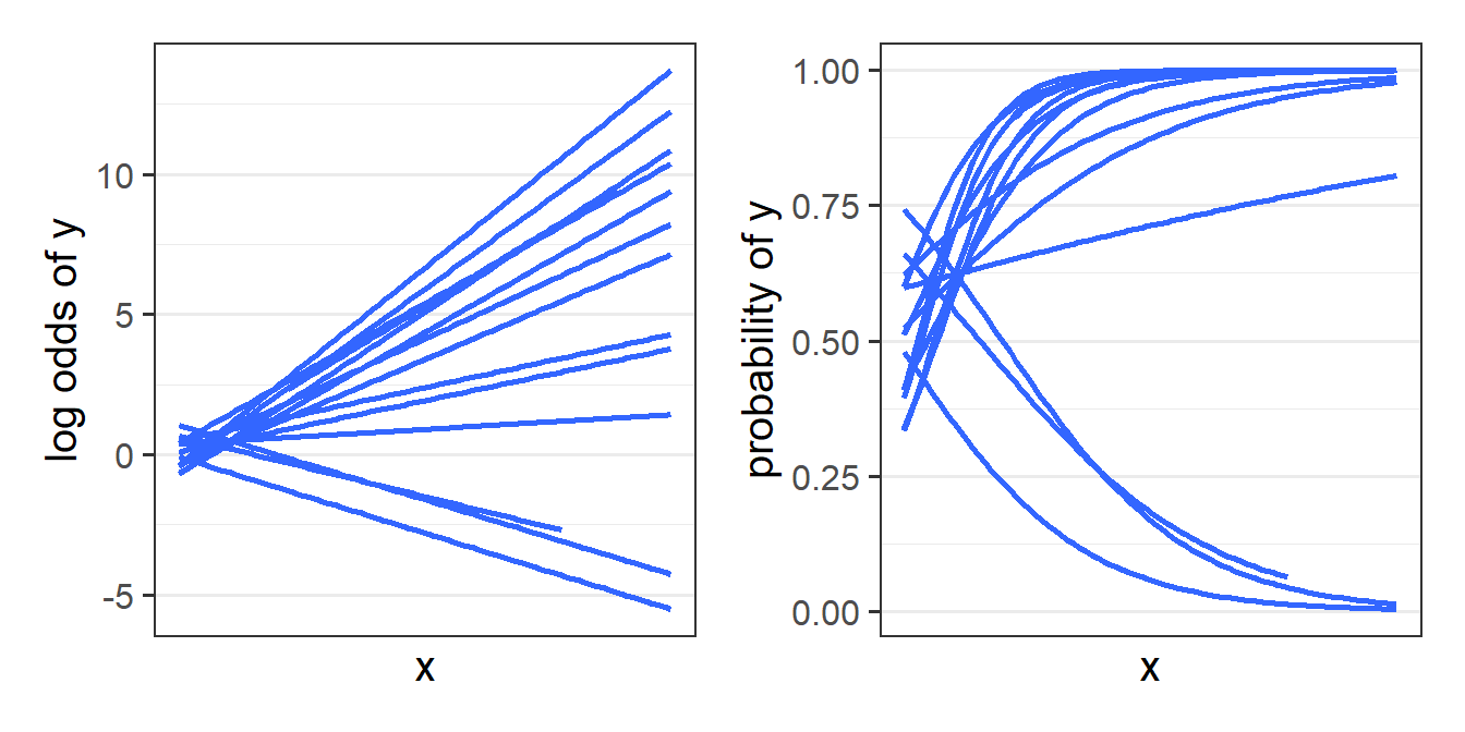
The same logic applies as it did for glm() where we are not modeling the outcome \(y\) directly, but via a mapping, or “link function”, which in this case is the logistic function. These model when we’re in the log-odds world have all the same properties (i.e. linear) that we have in lmer(). But converted back to the scale of our observed response (i.e. probabilities), we get the S-shaped curves that we saw with the glm() (as in Figure 1).
Beyond the material covered in , there are a few aspects of the logistic multilevel model that are worth commenting on.
Firstly, GLMMs (‘generalised linear mixed models’) can take more time to run (for bigger datasets we’re talking minutes, and sometimes even hours!).
Secondly, our choices of methods of inference (see 2A) are slightly different from what they were for lmer(). We continue to have the likelihood based methods as well as parametric bootstrapping (although this will more often result in computational issues with glmer). We also have the traditional \(z\)-statistics that have carried over from glm(). We can get confidence intervals that follow this same method by using confint(model, method="Wald"), which may often be preferred purely for the fact that they are quick!
Finally, one small but noteworthy feature of the logistic multilevel model is that our fixed effects coefficients, when translated back to odds ratios, represent “cluster specific” effects of a predictor:
- For a linear multilevel model:
lmer(y ~ x + (1 + x | cluster)), the fixed effect of \(x\) gives the change in the \(y\) when \(x\) is increased by one unit, averaged across clusters - For a logistic multilevel model:
glmer(ybin ~ x + (1 + x | cluster), family=binomial), the odds ratio for \(x\) -exp(fixef(model))- gives the multiplicative change in odds of \(y\) when \(x\) is increased by one unit for a particular cluster.
This becomes important when deciding if we want to estimate outcomes for individual clusters, or estimate group effects (in which case a mixed model might not be best).
Linear
consider a linear multilevel model:
lmer(respiratory_rate ~ treatment + (1|hospital))
Imagine two patients from different hospitals. One has a treatment, one does not.
- patient \(j\) from hospital \(i\) is “control”
- patient \(j'\) from hospital \(i'\) is “treatment”
The difference in estimated outcome between patient \(j\) and patient \(j'\) is the “the effect of having treatment” plus the distance in random deviations between hospitals \(i\) and \(i'\)
model for patient \(j\) from hospital \(i\)
\(\hat{y}_{ij} = (\gamma_{00} + \zeta_{0i}) + b_1 (Treatment_{ij} = 0)\)
model for patient \(j'\) from hospital \(i'\)
\(\hat{y}_{i'j'} = (\gamma_{00} + \zeta_{0i'}) + b_1 (Treatment_{i'j'} = 1)\)
difference:
\(\hat{y}_{i'j'} - \hat{y}_{ij} = b_1 + (\zeta_{0i'} - \zeta_{0i}) = b_1\)
Because \(\zeta \sim N(0,\sigma_\zeta)\), the differences between all different \(\zeta_{0i'} - \zeta_{0i}\) average out to be 0.
Logistic
Now consider a logistic multilevel model:
glmer(needs_operation ~ treatment + (1|hospital), family="binomial")
Imagine two patients from different hospitals. One has a treatment, one does not.
- patient \(j\) from hospital \(i\) is “control”
- patient \(j'\) from hospital \(i'\) is “treatment”
The difference in probability of outcome between patient \(j\) and patient \(j'\) is the “the effect of having treatment” plus the distance in random deviations between hospitals \(i\) and \(i'\)
model for patient \(j\) from hospital \(i\)
\(log \left( \frac{p_{ij}}{1 - p_{ij}} \right) = (\gamma_{00} + \zeta_{0i}) + b_1 (Treatment_{ij} = 0)\)
model for patient \(j'\) from hospital \(i'\)
\(log \left( \frac{p_{i'j'}}{1 - p_{i'j'}} \right) = (\gamma_{00} + \zeta_{0i'}) + b_1 (Treatment_{i'j'} = 1)\)
difference (log odds):
\(log \left( \frac{p_{i'j'}}{1 - p_{i'j'}} \right) - log \left( \frac{p_{ij}}{1 - p_{ij}} \right) = b_1 + (\zeta_{0i'} - \zeta_{0i})\)
difference (odds ratio):
\(\frac{p_{i'j'}/(1 - p_{i'j'})}{p_{ij}/(1 - p_{ij})} = e^{b_1 + (\zeta_{0i'} - \zeta_{0i})} \neq e^{b_1}\)
Hence, the interpretation of \(e^{b_1}\) is not the odds ratio for the effect of treatment “averaged over hospitals”, but rather for patients from the same hospital.
Example
Data: monkeystatus.csv
Our primate researchers have been busy collecting more data. They have given a sample of Rhesus Macaques various problems to solve in order to receive treats. Troops of Macaques have a complex social structure, but adult monkeys tend can be loosely categorised as having either a “dominant” or “subordinate” status. The monkeys in our sample are either adolescent monkeys, subordinate adults, or dominant adults. Each monkey attempted various problems before they got bored/distracted/full of treats. Each problems were classed as either “easy” or “difficult”, and the researchers recorded whether or not the monkey solved each problem.
We’re interested in how the social status of monkeys is associated with the ability to solve problems.
The data is available at https://uoepsy.github.io/data/msmr_monkeystatus.csv.
getting to know my monkeys
We know from the study background that we have a series group of monkeys who have each attempted to solve some problems. If we look at our data, we can see that it is already in long format, in that each row represents the lowest unit of observation (a single problem attempted). We also have the variable monkeyID which indicates what monkey each problem has been attempted by. We can see the status of each monkey, and the difficulty of each task, along with whether it was solved:
library(tidyverse)
library(lme4)
mstat <- read_csv("https://uoepsy.github.io/data/msmr_monkeystatus.csv")
head(mstat)
# A tibble: 6 × 4
status difficulty monkeyID solved
<chr> <chr> <chr> <dbl>
1 subordinate easy Seunghoo 1
2 subordinate easy Seunghoo 0
3 subordinate difficult Seunghoo 0
4 subordinate easy Seunghoo 1
5 subordinate difficult Seunghoo 0
6 subordinate easy Seunghoo 1We can do some quick exploring to see how many monkeys we have (50), and how many problems each one attempted (min = 3, max = 11:
mstat |>
  count(monkeyID) |> # count the monkeys!
  summary()
monkeyID n
Length:50 Min. : 3.00
Class :character 1st Qu.: 6.25
Mode :character Median : 8.00
Mean : 7.94
3rd Qu.:10.00
Max. :11.00 Let’s also see how many monkeys of different statuses we have in our sample:
mstat |>
  group_by(status) |> # group statuses
  summarise(
    # count the distinct monkeys
    nmonkey = n_distinct(monkeyID)
  )
# A tibble: 3 × 2
status nmonkey
<chr> <int>
1 adolescent 16
2 dominant 23
3 subordinate 11It’s often worth plotting as much as you can to get to a sense of what we’re working with. Here are the counts of easy/difficult problems that each monkey attempted. We can see that Richard only did difficult problems, and Nadheera only did easy ones, but most of the monkeys did both types of problem.
# which monkeys did what type of problems?
mstat |> count(status, monkeyID, difficulty) |>
  ggplot(aes(x=difficulty,y=n, fill=status))+
  geom_col()+
  facet_wrap(~monkeyID) +
  scale_x_discrete(labels=abbreviate) +
  theme(legend.position = "bottom")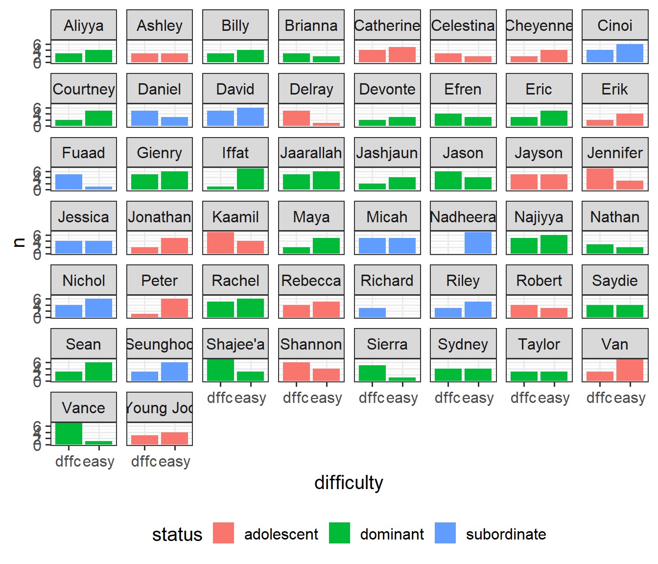
When working with binary outcomes, it’s often useful to calculate and plot proportions. In this case, the proportions of problems solved for each status of monkey. At first glance it looks like “subordinate” monkeys solve more problems, and adolescents solve fewer (makes sense - they’re still learning!).
# a quick look at proportions of problems solved:
ggplot(mstat, aes(x=difficulty, y=solved,
                       col=status))+
  stat_summary(geom="pointrange",size=1)+
  facet_wrap(~status)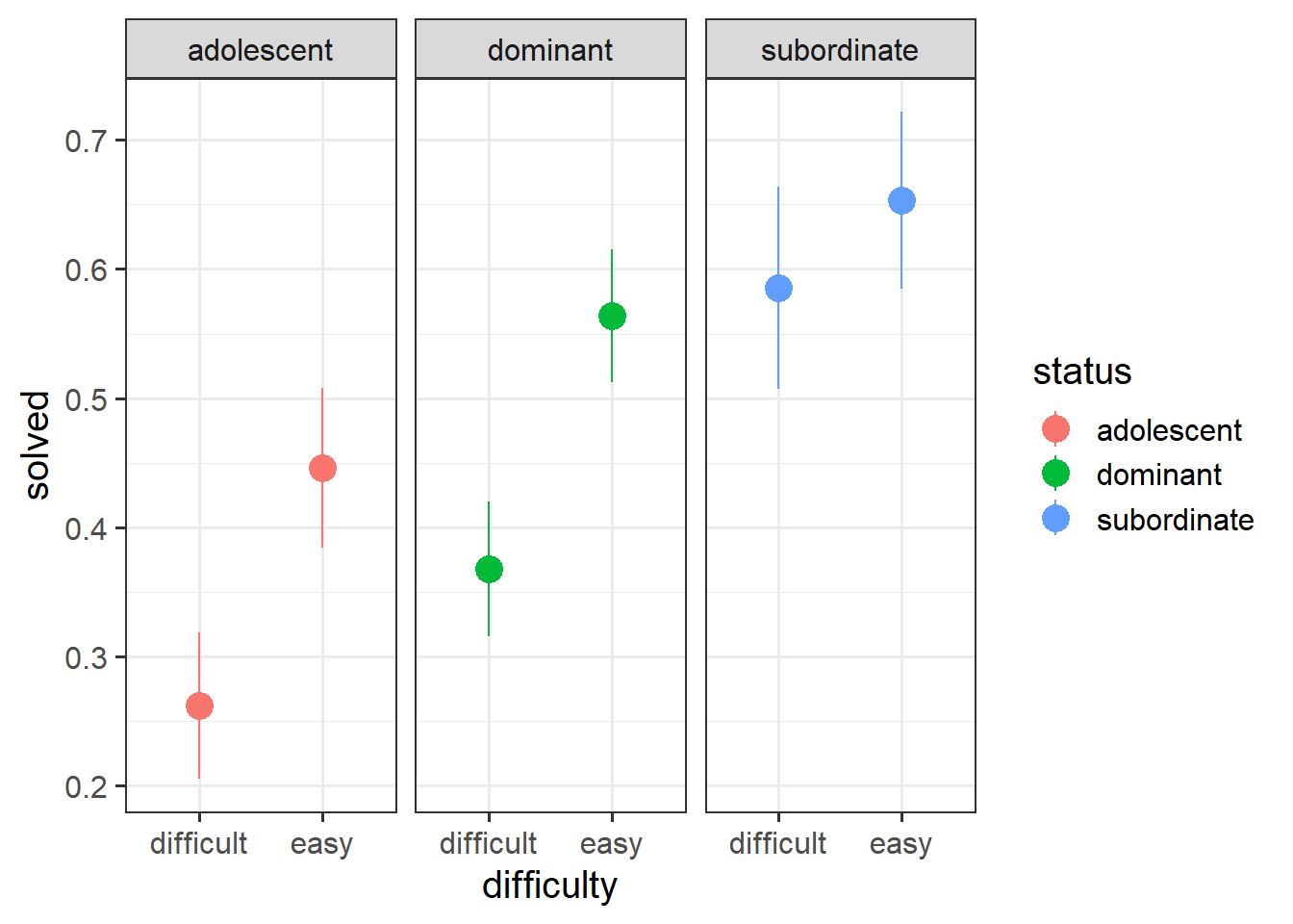
models of monkeys
Now we come to fitting our model.
Recall that we are interested in how the ability to solve problems differs between monkeys of different statuses. It’s very likely that difficulty of a problem is going to influence that it is solved, so we’ll control for difficulty.
glmer(solved ~ difficulty + status +
      ...
      data = mstat, family = binomial)
We know that we have multiple datapoints for each monkey, and it also makes sense that there will be monkey-to-monkey variability in the ability to solve problems (e.g. Brianna may be more likely to solve problems than Jonathan).
glmer(solved ~ difficulty + status +
      (1 + ... | monkeyID),
      data = mstat, family = binomial)
Finally, it also makes sense that effects of problem-difficulty might vary by monkey (e.g., if Brianna is just really good at solving problems, problem-difficulty might not make much difference. Whereas if Jonathan is struggling with the easy problems, he’s likely to really really struggle with the difficult ones!).
First, we’ll relevel the difficulty variable so that the reference level is “easy”:
mstat <- mstat |> mutate(
  difficulty = fct_relevel(factor(difficulty), "easy")
)
and fit our model:
mmod <- glmer(solved ~ difficulty + status +
      (1 + difficulty | monkeyID),
      data = mstat, family = binomial)
summary(mmod)
Generalized linear mixed model fit by maximum likelihood (Laplace
Approximation) [glmerMod]
Family: binomial ( logit )
Formula: solved ~ difficulty + status + (1 + difficulty | monkeyID)
Data: mstat
AIC BIC logLik deviance df.resid
503.7 531.6 -244.8 489.7 390
Scaled residuals:
Min 1Q Median 3Q Max
-1.9358 -0.6325 -0.3975 0.6748 2.5160
Random effects:
Groups Name Variance Std.Dev. Corr
monkeyID (Intercept) 1.551 1.246
difficultydifficult 1.371 1.171 -0.44
Number of obs: 397, groups: monkeyID, 50
Fixed effects:
Estimate Std. Error z value Pr(>|z|)
(Intercept) -0.3945 0.3867 -1.020 0.30767
difficultydifficult -0.8586 0.3053 -2.812 0.00492 **
statusdominant 0.6682 0.4714 1.417 0.15637
statussubordinate 1.4596 0.5692 2.564 0.01033 *
---
Signif. codes: 0 '***' 0.001 '**' 0.01 '*' 0.05 '.' 0.1 ' ' 1
Correlation of Fixed Effects:
(Intr) dffclt sttsdm
dffcltydffc -0.333
statusdmnnt -0.721 -0.031
statssbrdnt -0.594 -0.033 0.497test and visualisations of monkey status
To examine if monkey status has an effect, we can compare with the model without status:
Code
mmod0 <- glmer(solved ~ difficulty +
      (1 + difficulty | monkeyID),
      data = mstat, family = binomial)
anova(mmod0, mmod)
Data: mstat
Models:
mmod0: solved ~ difficulty + (1 + difficulty | monkeyID)
mmod: solved ~ difficulty + status + (1 + difficulty | monkeyID)
npar AIC BIC logLik deviance Chisq Df Pr(>Chisq)
mmod0 5 506.13 526.05 -248.07 496.13
mmod 7 503.70 531.58 -244.85 489.70 6.4367 2 0.04002 *
---
Signif. codes: 0 '***' 0.001 '**' 0.01 '*' 0.05 '.' 0.1 ' ' 1And we can see that the status of monkeys is associated with differences in the probability of successful problem solving (\(\chi^2(2)\) = 6.44, p < 0.05).
And if we want to visualise the relevant effect, we can (as we did with glm()) plot on the predicted probability scale, which is much easier to interpret:
Code
library(effects)
effect(term=c("status","difficulty"), mod=mmod) |>
  as.data.frame() |>
  ggplot(aes(x=difficulty, y=fit))+
  geom_pointrange(aes(ymin=lower,ymax=upper, col=status),
                  size=1, lwd=1,
                  position=position_dodge(width=.3)) +
  labs(x = "problem difficulty", y = "predicted probability")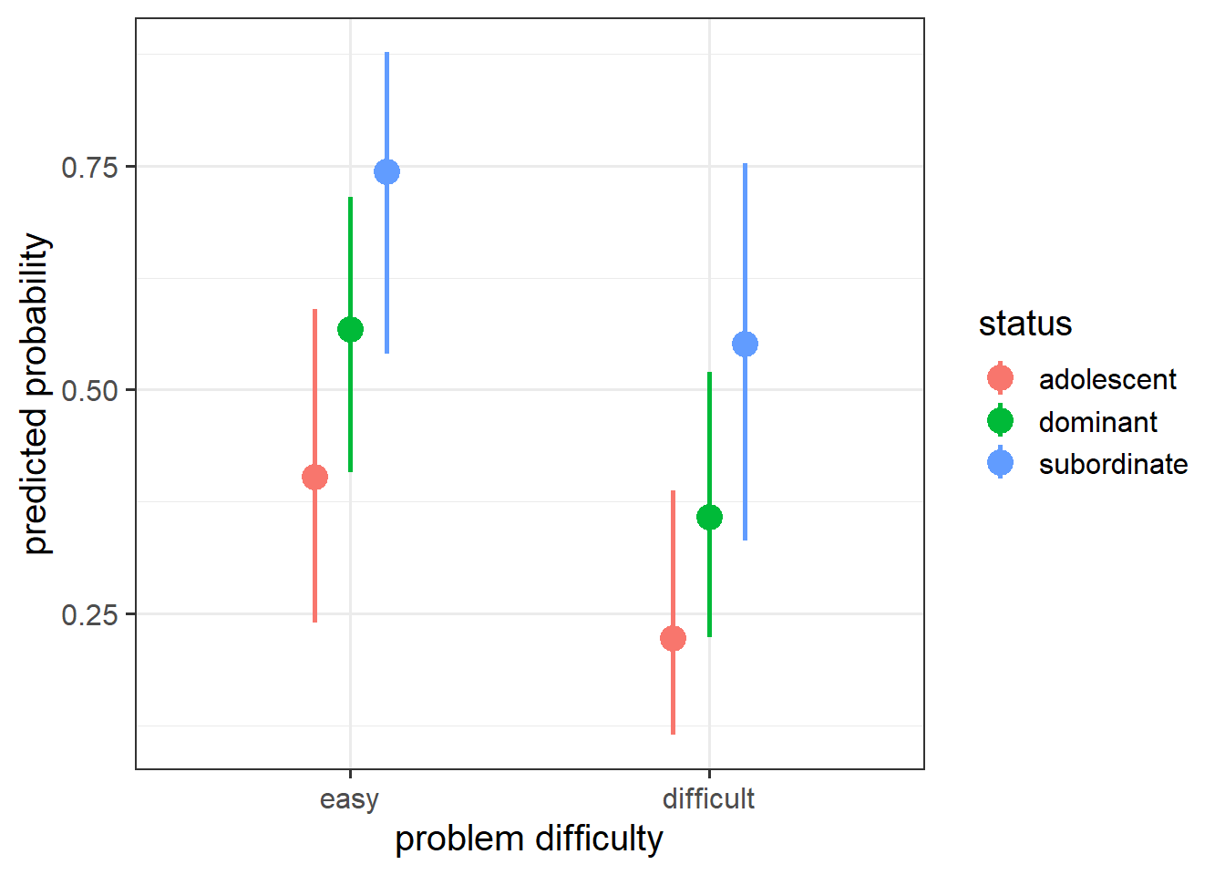
interpretation
And just with the single level logistic models, our fixed effects can be converted to odds ratios (OR), by exponentiation:
cbind(
  fixef(mmod), # the fixed effects
  confint(mmod, method="Wald", parm="beta_") # Wald CIs for fixed effects
) |>
  exp()
2.5 % 97.5 %
(Intercept) 0.6740221 0.3158658 1.4382872
difficultydifficult 0.4237565 0.2329242 0.7709359
statusdominant 1.9506650 0.7743099 4.9141746
statussubordinate 4.3042614 1.4106434 13.1334867| term | est | OR | OR interpretation |
|---|---|---|---|
| (Intercept) | -0.39 | 0.67 | estimated odds of an adolescent monkey solving an easy problem |
| difficultydifficult | -0.86 | 0.42 | odds of successful problem solving are more than halved (0.42 times the odds) when a given monkey moves from an easy to a difficult problem |
| statusdominant | 0.67 | 1.95 | odds of success would be almost doubled (1.95 times the odds) if a monkey were to change from adolescent to dominant status (NB this is non-significant) |
| statussubordinate | 1.46 | 4.30 | odds of success would quadruple (4.3 times the odds) if a monkey were to change from adolescent to subordinate status |
Side note
Contrast this with what we would get from a linear multilevel model. If we were instead modelling a “problem score” with lmer(), rather than “solved yes/no” with glmer(), our coefficients would be interpreted as the estimated difference in scores between adolescent and subordinate monkeys.
Note that estimating differences between groups is not quite the same idea as estimating the effect “if a particular monkey changed from adolescent to subordinate”. In the linear world, these two things are the same, but our odds ratios give us only the latter.
MLMs for Longitudinal Data
Multilevel models are perfectly geared towards dealing with longitudinal data, which can be framed as having essentially the same hierarchical structure as “children in schools”, or “observations within participant”.
The only difference is that in longitudinal data, the repeated measurements within a participant are ordered according to time. For instance, this could apply to anything from studying people over decades as they age to studying eye movements across the 1 second presentation of a spoken word.
As with all applications of multilevel models, we will want our data in long format, so it is usually going to look something like this:
    y time person ...  ...
1   ?    1      1  ...   ...
2   ?    2      1  ...   ...
3 ...  ...    ...  ...   ...
4 ...  ...    ...  ...   ...
5   ?    1      2  ...   ...
6   ?    2      2  ...   ...
7 ...  ...    ...  ...   ...
We are treating time as continuous here, which has some great benefits - we don’t need to have seen everyone at every timepoint, nor do we even need to have everyone with regularly spaced intervals (although knowing the chronology is important for decisions about the shape of trajectory we might want to fit (more on that next week!)).
Given the variables above, you might be able to guess the basic form that our models are going to take in order to assess “change over time”.
Regressing the outcome variable on to our time variable gives us an estimate of the trajectory - i.e. how much the outcome changes with every 1 additional unit of time. Furthermore, we can fit random slopes of time in order to model how people2 can vary in the trajectory.
lmer(y ~ 1 + time + (1 + time | person), ...)And we can fit interactions between predictors and time (y ~ time * x) to ask questions such as whether different groups have different trajectories of y, or whether the association between x and y changes over time (x can also be something that changes over time!). For instance, we can use multilevel models to address question such as does the development of reading ability differ between monolingual and bilingual children? Does the association between physical activity and positive mood change as we age? Do people look at the more unusual of two objects following a speech disfluency?
Example
Data: mindfuldecline.csv
A study is interested in examining whether engaging in mindfulness can prevent cognitive decline in older adults. They recruit a sample of 20 participants at age 60, and administer the Addenbrooke’s Cognitive Examination (ACE) every 2 years (until participants were aged 78). Half of the participants complete weekly mindfulness sessions, while the remaining participants did not.
The data are available at: https://uoepsy.github.io/data/msmr_mindfuldecline.csv.
| variable | description |
|---|---|
| ppt | Participant Identifier |
| condition | Whether the participant engages in mindfulness or not (control/mindfulness) |
| study_visit | Study Visit Number (1 - 10) |
| age | Age (in years) at study visit |
| ACE | Addenbrooke's Cognitive Examination Score. Scores can range from 0 to 100 |
| imp | Clinical diagnosis of cognitive impairment ('imp' = impaired, 'unimp' = unimpaired) |
exploring the data
library(tidyverse)
library(lme4)
mmd <- read_csv("https://uoepsy.github.io/data/msmr_mindfuldecline.csv")
head(mmd)
# A tibble: 6 × 6
ppt condition study_visit age ACE imp
<chr> <chr> <dbl> <dbl> <dbl> <chr>
1 PPT_1 control 1 60 84.5 unimp
2 PPT_1 control 2 62 85.6 imp
3 PPT_1 control 3 64 84.5 imp
4 PPT_1 control 4 66 83.1 imp
5 PPT_1 control 5 68 82.3 imp
6 PPT_1 control 6 70 83.3 imp How many participants in each condition? We know from the description there should be 10 in each, but lets check!
mmd |>
  group_by(condition) |>
  summarise(
    n_ppt = n_distinct(ppt)
  )
# A tibble: 2 × 2
condition n_ppt
<chr> <int>
1 control 10
2 mindfulness 10How many observations does each participant have? With only 20 participants, we could go straight to plotting as a way of getting lots of information all at once. From the plot below, we can see that on the whole participants’ cognitive scores tend to decrease. Most participants have data at every time point, but 4 or 5 people are missing a few. The control participants look (to me) like they have a slightly steeper decline than the mindfulness group:
ggplot(mmd, aes(x = age, y = ACE, col = condition)) +
  geom_point() +
  geom_line(aes(group=ppt), alpha=.4)+
  facet_wrap(~ppt)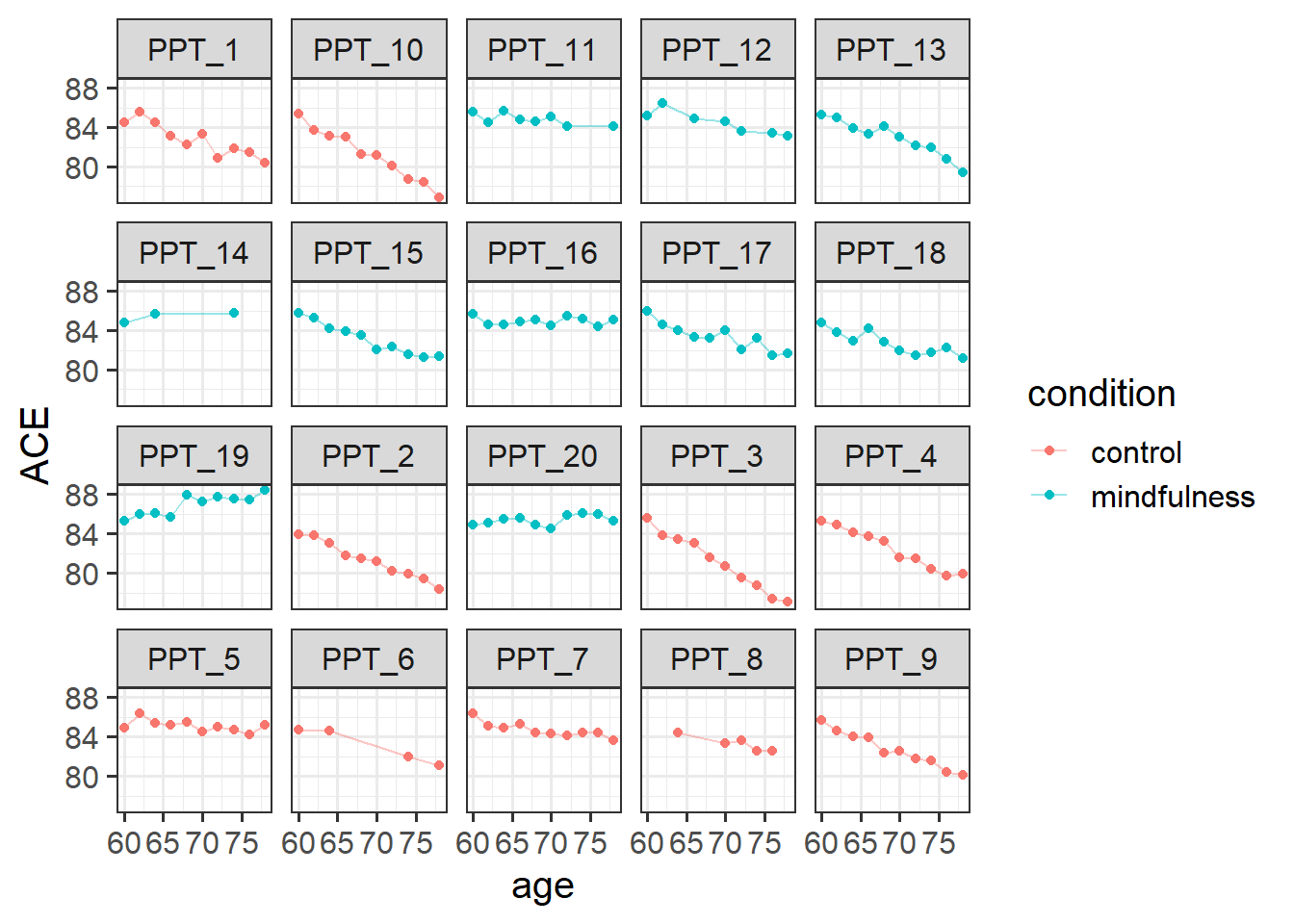
modelling change over time
Initially, we’ll just model how cognition changes over time across our entire sample (i.e. ignoring the condition the participants are in). Note that both the variables study_visit and age represent exactly the same information (time), so we have a choice of which one to use.
As it is, the age variable we have starts at 60 and goes up to 78 or so.
If we try and use this in a model, we get an error!
mod1 <- lmer(ACE ~ 1 + age +
               (1 + age | ppt),
             data = mmd)
Model failed to converge with max|grad| = 0.366837 (tol = 0.002, component 1)
This is because of the fact that intercepts and slopes are inherently dependent upon one another. Remember that the intercept is “when all predictors are zero”. So in this case it is the estimate cognition of new-born babies. But all our data comes from people who are 65+ years old!
This means that trying to fit (1 + age | ppt) will try to estimate the variability in people’s change in cognition over time, and the variability in cognition at age zero. As we can see in Figure 2, because the intercept is so far away from the data, the angle of each persons’ slope has a huge influence over where their intercept is. The more upwards a persons’ slope is, the lower down their intercept is.
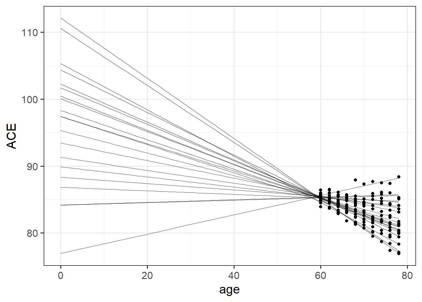
This results in issues for estimating our model, because the intercepts and slopes are perfectly correlated! The estimation process has hit a boundary (a perfect correlation):
VarCorr(mod1) Groups Name Std.Dev. Corr
ppt (Intercept) 7.51567
age 0.12696 -0.999
Residual 0.51536 So what we can do is either center age on 60 (so that the random intercept is the estimated variability in cognition at aged 60, i.e. the start of the study), or use the study_visit variable.
Either will do, we just need to remember the units they are measured in!
Let’s center age on 60:
mmd$ageC <- mmd$age-60And fit our model:
mod1 <- lmer(ACE ~ 1 + ageC +
               (1 + ageC | ppt),
             data = mmd)
From our fixed effects, we can see that scores on the ACE tend to decrease by about 0.18 for every 1 year older people get (as a very rough rule of thumb, \(t\) statistics that are \(>|2\text{-ish}|\) are probably going to be significant when assessed properly).
summary(mod1)...
Fixed effects:
Estimate Std. Error t value
(Intercept) 85.22558 0.10198 835.735
ageC -0.17938 0.03666 -4.893We’re now ready to add in group differences in their trajectories of cognition:
mod2 <- lmer(ACE ~ 1 + ageC * condition +
               (1 + ageC | ppt),
             data = mmd)
From this model, we can see that for the control group the estimated score on the ACE at age 60 is 85 (that’s the (Intercept)). For these participants, scores are estimated to decrease by -0.27 points every year (that’s the slope of ageC). For the participants in the mindfulness condition, they do not score significantly differently from the control group at age 60 (the condition [mindfulness] coefficient). For the mindfulness group, there is a reduction in the decline of cognition compared to the control group, such that this group decline 0.17 less than the control group every year.
(note, there are always lots of ways to frame interactions. A “reduction in decline” feels most appropriate to me here)
Given that we have a fairly small number of clusters here (20 participants), Kenward Rogers is a good method of inference as it allows us to use REML (meaning unbiased estimates of the random effect variances) and it includes a small sample adjustment to our standard errors.
library(parameters)
model_parameters(mod2, ci_method="kr", ci_random=FALSE)
# Fixed Effects
Parameter | Coefficient | SE | 95% CI | t | df | p
----------------------------------------------------------------------------------------------
(Intercept) | 85.20 | 0.15 | [84.89, 85.52] | 568.00 | 17.75 | < .001
ageC | -0.27 | 0.04 | [-0.36, -0.17] | -5.93 | 17.95 | < .001
condition [mindfulness] | 0.05 | 0.21 | [-0.39, 0.49] | 0.23 | 17.49 | 0.821
ageC × condition [mindfulness] | 0.17 | 0.06 | [ 0.04, 0.31] | 2.73 | 17.99 | 0.014
# Random Effects
Parameter | Coefficient
---------------------------------------
SD (Intercept: ppt) | 0.35
SD (ageC: ppt) | 0.14
Cor (Intercept~ageC: ppt) | 0.26
SD (Residual) | 0.49From those parameters and our interpretation above, we are able to start putting a picture together - two groups that start at the same point, one goes less steeply down over time than the other.
And that’s exactly what we see when we visualise those fixed effects:
Code
library(effects)
effect(term="ageC*condition", mod=mod2, xlevels=10) |>
  as.data.frame() |>
  ggplot(aes(x=ageC+60,y=fit,
             ymin=lower,ymax=upper,
             col=condition, fill = condition))+
  geom_line(lwd=1)+
  geom_ribbon(alpha=.2, col=NA) +
  scale_color_manual(values=c("#a64bb0","#82b69b"))+
  scale_fill_manual(values=c("#a64bb0","#82b69b"))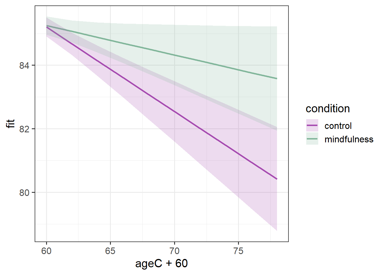
Sometimes it is more helpful for a reader if we add in the actual observed trajectories to these plots. To do so, we need to combine two data sources - the fixed effects estimation from effect(), and the data itself:
Code
ploteff <- effect(term="ageC*condition", mod=mod2, xlevels=10) |>
  as.data.frame()

mmd |>
  ggplot(aes(x=ageC+60,col=condition,fill=condition))+
  geom_line(aes(y=ACE,group=ppt), alpha=.4) +
  geom_line(data = ploteff, aes(y=fit), lwd=1)+
  geom_ribbon(data = ploteff, aes(y=fit,ymin=lower,ymax=upper),
              alpha=.2, col=NA) +
  scale_color_manual(values=c("#a64bb0","#82b69b"))+
  scale_fill_manual(values=c("#a64bb0","#82b69b"))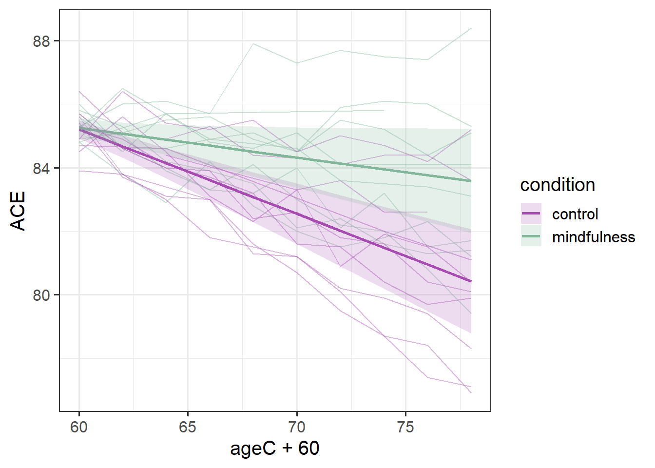
This plot gives us more a lot more context. To a lay reader, our initial plot potentially could be interpreted as if we would expect every person’s cognitive trajectories to fall in the blue and red bands. But those bands are representing the uncertainty in the fixed effects - i.e. the uncertainty in the average persons’ trajectory. When we add in the observed trajectories, we see the variability in people’s trajectories (one person even goes up over time!).
Our model represents this variability in the random effects part. While the estimated average slope is -0.27 for the control group (and -0.27+0.17=-0.09 for the mindfulness group), people are estimated to vary in their slopes with a standard deviation of 0.14 (remember we can extract this info using VarCorr(), or just look in the output of summary(model)).
VarCorr(mod2) Groups Name Std.Dev. Corr
ppt (Intercept) 0.34615
ageC 0.13866 0.260
Residual 0.49450 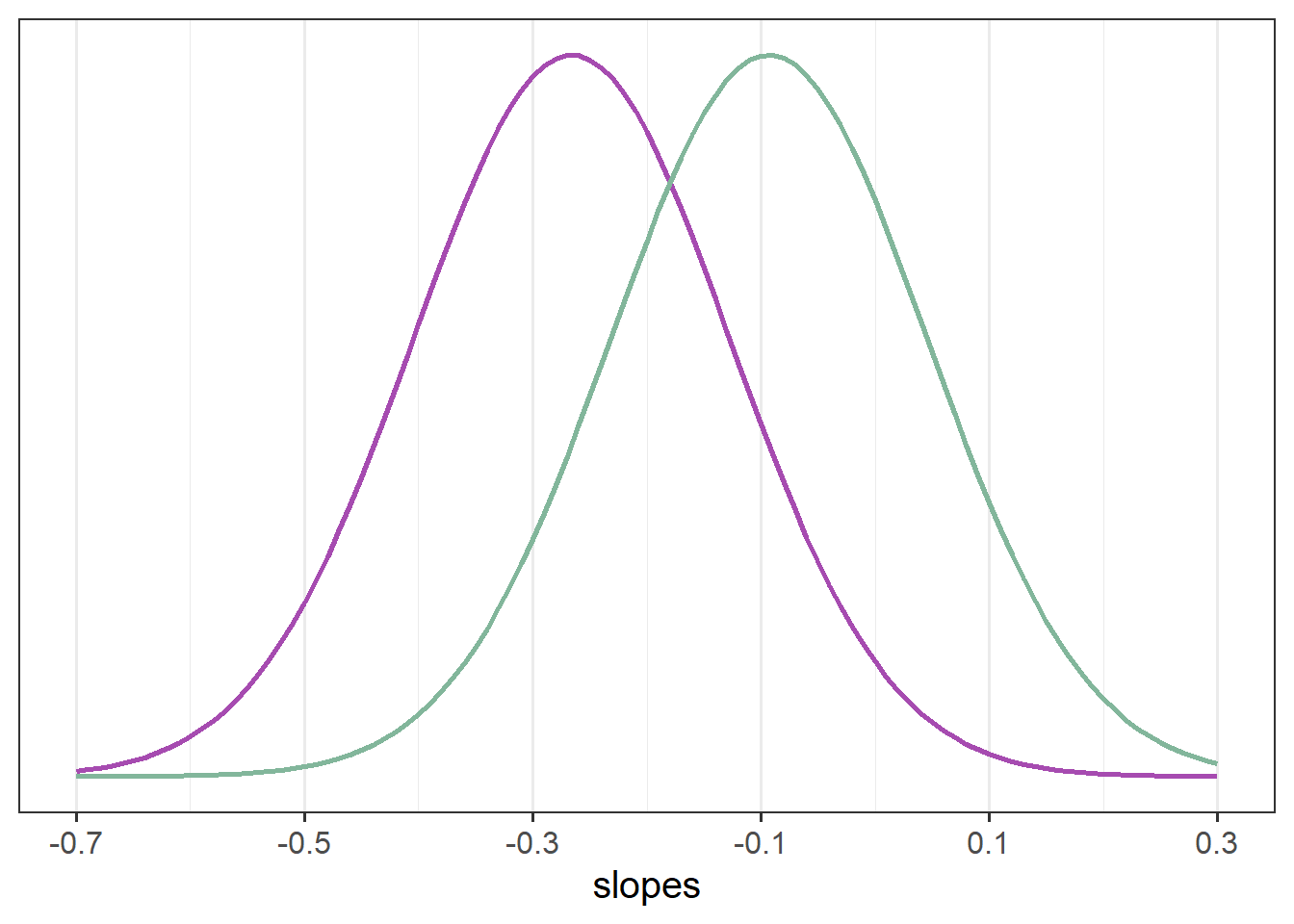
If you think about what this means - it means that some participants we would expect to actually increase in their slopes. If we have a normal distribution with a mean of -0.3 or -0.09 and a standard distribution of 0.14, then we would expect some values to to positive (see e.g., Figure 3).