4A: Random Effect Structures

This reading:

• extending the multilevel model to encompass more complex random effect structures

• model building and common issues

“random effects”

So far, we’ve fitted various multilevel models that have had grouping structures such as:

• each observation is a child, and children are grouped into schools
• each observation is an individual trial or assessment, and multiple observations come from each participants
• each observation is a single timepoint, and we have multiple timepoints for each participant

In all of these, we have been specifying models with a random effect structure that takes the form (.... | g).

We’re now going to move to look at how multilevel modelling can capture more complex structures - when there is more than just the one grouping variable.

a small note on how people use the term “random effects”

People often use the term “random effects” to collectively refer to all of the stuff we’re putting in the brakects of lmer():

\[ \text{... + }\underbrace{\text{(random intercept + random slopes | grouping structure)}}_{\text{random effects}} \]

People will use different phrases to refer to individual random intercepts or slopes, such as:

• “random effects of x by g” to refer to ... + x | g)
• “by-g random effects of x” to refer to ... + x | g)
• “random effects of x for g” to refer to ... + x | g)
• “random effect for/of g” to refer to (1 | g)

These are all really trying to just different ways to say that a model allows [insert-parameter-here] to be different for each group of g, and that it estimates their variance.

Nested

The same principle we have seen for models with 2 levels can be extended to situations in which those level 2 clusters are themselves grouped in to higher level clusters.

For instance:

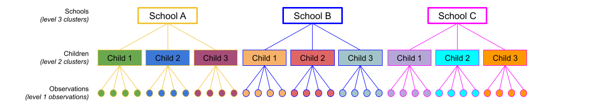
• each observation is a child, and children are grouped into schools. Schools are nested within districts.
  
• each observation is an individual assessment, and we have multiple assessments for each patient, and patients are nested within hospitals.
• each observation is an individual timepoint, and we have multiple timepoint per child. children are nested within schools

This sort of structure is referred to as “nested” in that at each level, individual units belong to only one of the higher up units. For instance, in a “observations within children within schools” structure, each observation belongs to only one child, and each child is at only one school. You can see this idea in Figure 1

Figure 1: A ‘nested’ structure, in which each level 1 unit belongs to a single level 2 unit, and each level 2 unit belongs to a single level 3 unit

In R, we can specify a nested structure using:

... + (1 + ... | school) + (1 + .... | school:child)

This specifies that things can vary between schools and that things can also vary between the children within the schools.

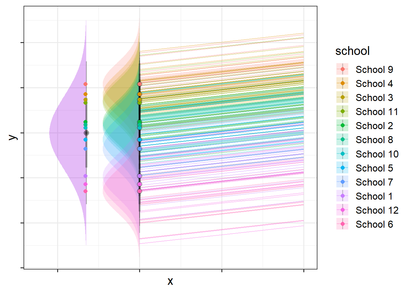
So (1 | school) + (1 | school:child) means that the intercept varies by school (some schools have a higher \(y\), some have lower), and also by the children within the schools (some children have a higher \(y\) for the school, some have lower).

You might think of this as the variance in school intercepts (width of purple distribution in Figure 2) and the variance in child intercepts around their school average (width of the right-hand distributions in Figure 2). In Figure 2 below there is a lot of school-level variation, and less child-level variation, but you could just as likely have a situation in which children that vary a lot and schools vary less.

Figure 2: Lines for each child from 12 Schools. Purple distribution shows school-level variance in intercepts. Distributions to the right show the within-school child-level variance in intercepts

a shortcut

In lme4, there is a shortcut for writing nested random effects that uses the / to specify higher/lower level of nesting.

For instance,
(1 + .... | school/child)
is the same thing as
(1 + ... | school) + (1 + .... | school:child)

This shortcut has a bit of a disadvantage in that it means all the same random slopes are fitted for schools and for children-within-schools, so often it is preferable to keep them separated out.

uniqueness of labels

If labels of children are unique to each school, e.g. the child variable has values like “school1_child1”, “school2_child2” etc., then school:child captures the same set of groups as child does, and therefore
(1 + ... | school) + (1 + .... | school:child)
is the same as
(1 + ... | school) + (1 + .... | child)

The risk of just specifying ... |child is that whether or not it gets at the correct groups depends on your labels.

in the summary() output of a multilevel model, immediately beneath the random effects it will show you how many groups. It’s always worth checking that these match with how many you would expect!

Crossed

Crossed structures are, in simplest terms, anything that is not nested. So if a unit of observation exists in more than one of another level, we have a crossed design - i.e. where there is not the same hierarchy to the structure.

For instance:

• Each observation is an assessment of a patient by a therapist. Patients see various therapists, and therapists see many different patients (patients and therapists are not nested)
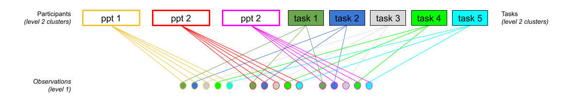
• Each observation is an individual trial, which will be one from a set of experimental items. All participants see all items, but all items are seen by all participants, so items and participants are not nested.

This sort of structure is referred to as “crossed” because of the lines crossing in such diagrams as in Figure 3. In Figure 3, observations can be grouped into tasks, but they can also be grouped into participants.

Figure 3: A ‘crossed’ structure

In R, we simply specify these as separate groupings

... + (1 + ... | participant) + (1 + .... | task)

This specifies that things can vary between participants, and that things can also vary between tasks.

So (1 | participant) + (1 | task) means that the intercept varies by participant (some people have a higher \(y\), some have lower),b and also by tasks (some tasks result in a higher \(y\), some lower).

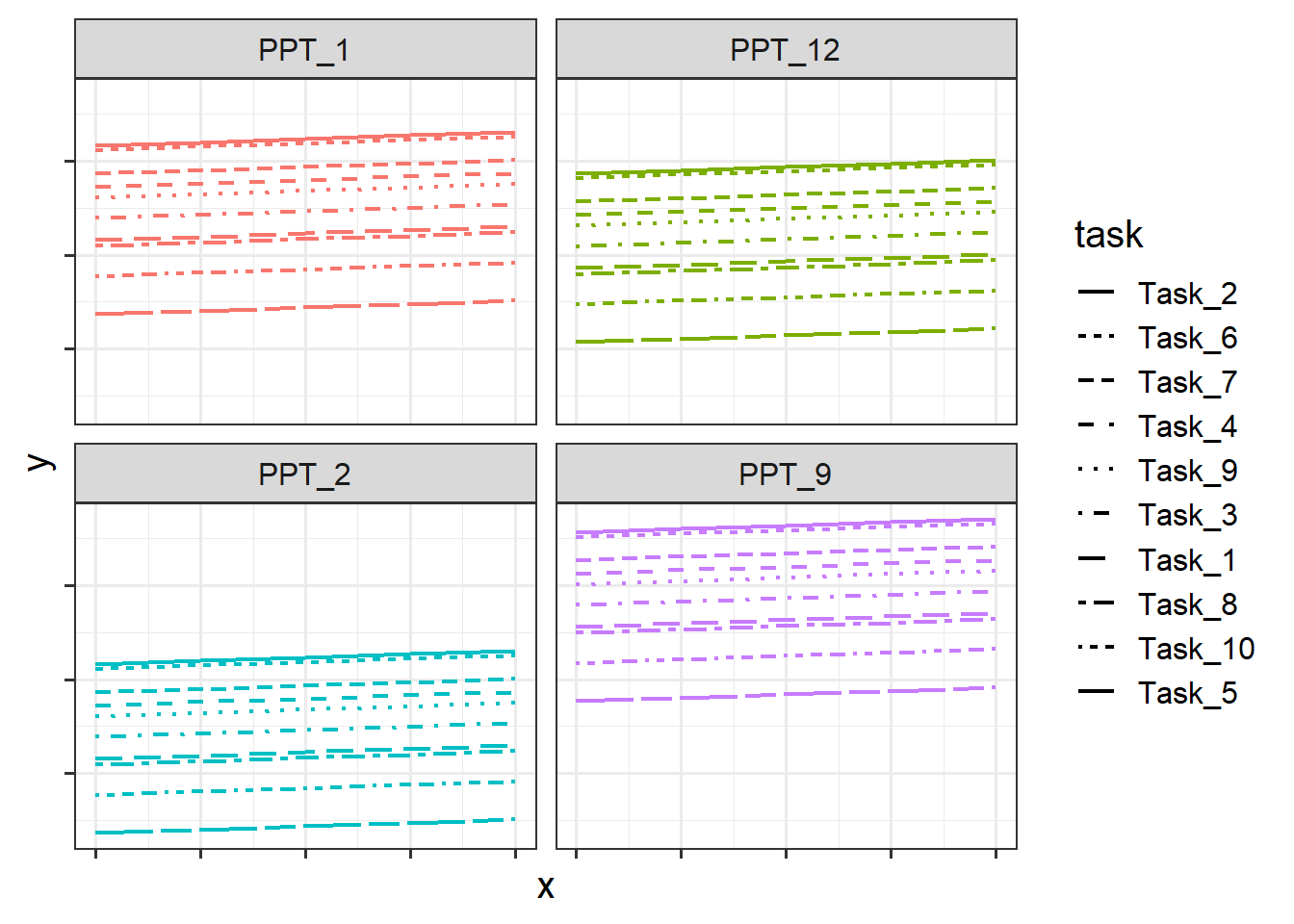
It’s a bit more difficult to visualise, but Figure 4 shows two independent distributions representing the intercept variance between Participants (left) and between Tasks (right).

Figure 4: A crossed design, with participant level variance (left) and task level variance (right)

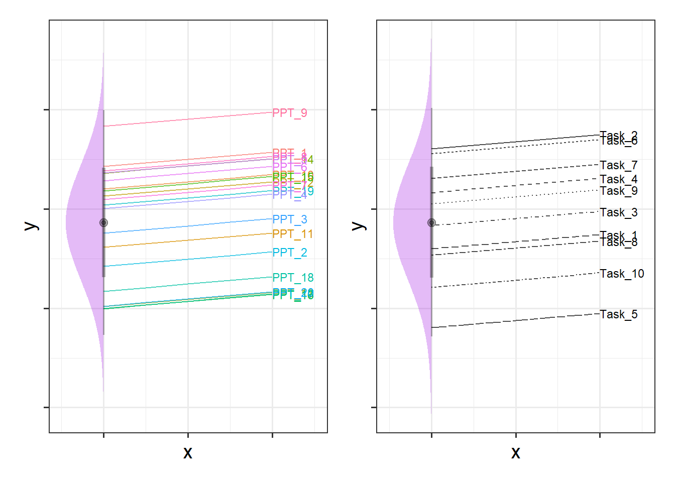
We can see in Figure 4, for instance, that “PPT_9” tends to have a higher \(y\), and that “Task_5” tends to have lower scores etc. Combined, these imply our model fitted values as shown for just 4 of the participants in Figure 5.

Figure 5: fitted values from a crossed design for a sample of 4 participants

Examples

Example 1: Two levels

Below is an example of a study that has a similar structure to those that we’ve seen thus far, in which we have just two levels (observations that are grouped in some way).

Study Design

Suppose, for instance, that we conducted an experiment on a sample of 20 staff members from the Psychology department to investigate effects of CBD consumption on stress over the course of the working week. Participants were randomly allocated to one of two conditions: the control group continued as normal, and the CBD group were given one CBD drink every day. Over the course of the working week (5 days) participants stress levels were measured using a self-report questionnaire.

We can see our data here:

psychstress <- read_csv("https://uoepsy.github.io/data/stressweek1.csv")
head(psychstress)

# A tibble: 6 × 6
  dept  pid   CBD   measure       day stress
  <chr> <chr> <chr> <chr>       <dbl>  <dbl>
1 Psych Holly N     Self-report     1 -0.417
2 Psych Holly N     Self-report     2  0.924
3 Psych Holly N     Self-report     3  0.634
4 Psych Holly N     Self-report     4  1.21 
5 Psych Holly N     Self-report     5  0.506
6 Psych Tom   Y     Self-report     1 -0.557

Plot

Code

# take the dataset, and make the x axis of our plot the 'day' variable, 
# and the y axis the 'stress' variable: 
# color everything by the CBD groups
ggplot(psychstress, aes(x = day, y = stress, col=CBD)) + 
  geom_point() + # add points to the plot
  geom_line() + # add lines to the plot
  facet_wrap(~pid) # split it by participant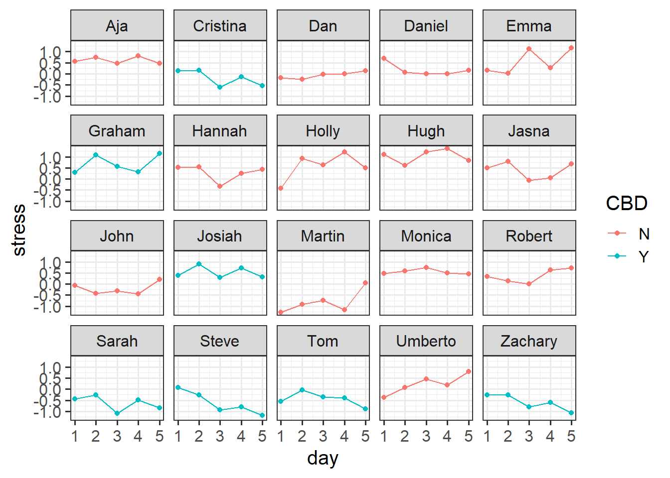

Model

We might fit a model that looks something like this:

Code

library(lme4)
# re-center 'day' so the intercept is day 1
psychstress$day <- psychstress$day-1 

# fit a model of stress over time: stress~day
# estimate differences between the groups in their stress change: day*CBD
# people vary in their overall stress levels: 1|pid
# people vary in their how stress changes over the week: day|pid
m2level <- lmer(stress ~ 1 + day * CBD + 
                  (1 + day | pid), data = psychstress)

Note that there is a line in the model summary output just below the random effects that shows us the information about the groups, telling us that we have 100 observations that are grouped into 20 different participants’.

summary(m2level)

Linear mixed model fit by REML ['lmerMod']
Formula: stress ~ 1 + day * CBD + (1 + day | pid)
   Data: psychstress

REML criterion at convergence: 127.7

Scaled residuals: 
     Min       1Q   Median       3Q      Max 
-2.17535 -0.65204 -0.02667  0.64622  1.81574 

Random effects:
 Groups   Name        Variance Std.Dev. Corr
 pid      (Intercept) 0.199441 0.44659      
          day         0.004328 0.06579  0.02
 Residual             0.112462 0.33535      
Number of obs: 100, groups:  pid, 20

Fixed effects:
            Estimate Std. Error t value
(Intercept)  0.13178    0.14329   0.920
day          0.07567    0.03461   2.186
CBDY        -0.08516    0.24221  -0.352
day:CBDY    -0.19128    0.05851  -3.270

Correlation of Fixed Effects:
         (Intr) day    CBDY  
day      -0.339              
CBDY     -0.592  0.201       
day:CBDY  0.201 -0.592 -0.339

Example 2: Three level Nested

Let’s suppose that instead of simply sampling 20 staff members from the Psychology department, we instead went out and sampled lots of people from different departments across the University. The dataset below contains not just our 20 Psychology staff members, but also data from 220 other people from departments such as History, Philosophy, Art, etc..

neststress <- read_csv("https://uoepsy.github.io/data/stressweek_nested.csv")
head(neststress)

# A tibble: 6 × 6
  dept  pid      CBD   measure       day stress
  <chr> <chr>    <chr> <chr>       <dbl>  <dbl>
1 CMVM  Ryan     Y     Self-report     1  0.933
2 CMVM  Ryan     Y     Self-report     2  0.997
3 CMVM  Ryan     Y     Self-report     3  0.408
4 CMVM  Ryan     Y     Self-report     4  0.581
5 CMVM  Ryan     Y     Self-report     5  0.442
6 CMVM  Nicholas Y     Self-report     1  0.138

In this case, we have observations that are grouped by participants, and those participants can be grouped into the department in which they work. Three levels of nesting!

You can see in the Figure 6 below that there is variation between departments (i.e. people working in Art are a bit more relaxed, Political Science and CMVM is stressful, etc), and then within each of those, there is variation between participants (i.e. some people working in Art are more stressed than other people in Art).

Code

ggplot(neststress, aes(x=day, y=stress,col=CBD))+
  # plot points
  geom_point()+
  # split by departments
  facet_wrap(~dept)+
  # make a line for each participant
  geom_line(aes(group=pid),alpha=.3)+ 
  # plot the mean and SE for each day.
  stat_summary(geom="pointrange",col="black")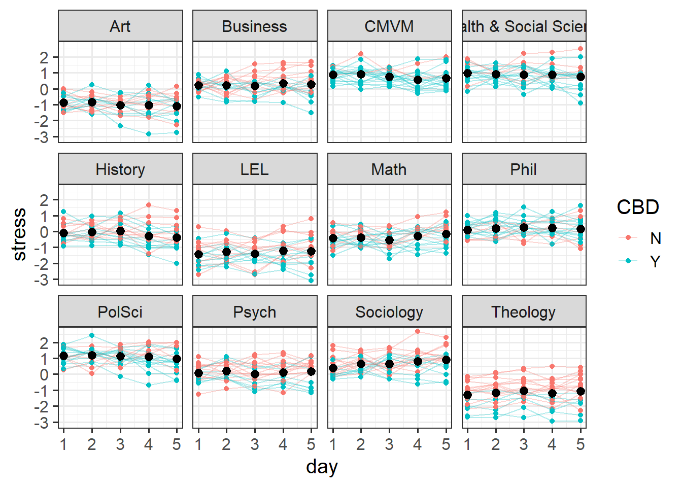

Figure 6: A longitudinal study in which participants are nested within department

To account for these multiple sources of variation, we can fit a model that says both ( ... | dept) (“things vary by department”) and ( ... | dept:pid) (“things vary by participants within departments”).

So a model might look something like this:

# re-center 'day' so the intercept is day 1
neststress$day <- neststress$day-1

mnest <- lmer(stress ~ 1 + day * CBD + 
                (1 + day * CBD | dept) +
                (1 + day | dept:pid), data = neststress)

Note that we can have different random slopes for departments vs those for participants. Our model above includes all random slopes that are feasible given the study design.

explanations of each random slope

• participants can vary in their baseline stress levels.
  • (1 | dept:pid)
• participants can vary in how stress changes over the week. e.g., some participants might get more stressed over the week, some might get less stressed
  • (days | dept:pid)
    
• participants cannot vary in how CBD changes their stress level. because each participant is either CBD or control, “the effect of CBD on stress” doesn’t exist for a single participant (and so can’t very between participants)
  • (CBD | dept:pid)
    
• participants cannot vary in how CBD affects their changes in stress over the week. For the same reason as above.
  • ( day*CBD | dept:pid)
• departments can vary in their baseline stress levels.
  • (1 | dept)
    
• departments can vary in how stress changes over the week.
  • (days | dept)
• departments can vary in how CBD changes stress levels. because each department contains some participants in the CBD group and some in the control group, “the effect of CBD on stress” does exist for a given department, and so could vary between departments. e.g. Philosophers taking CBD get really relaxed, but CBD doesn’t affect Mathematicians that much.
  • (CBD | dept)
    
• departments can vary in how CBD affects changes in stress over the week
  • ( day*CBD | dept)

Note that the above model is a singular fit, but it gives us a better place to start simplifying from. If we remove the day*CBD interaction in the by-department random effects, we get a model that converges:

mnest2 <- lmer(stress ~ 1 + day * CBD + 
                (1 + day + CBD | dept) +
                (1 + day | dept:pid), data = neststress)

And plot our fitted values

Code

library(broom.mixed)
augment(mnest2) |> 
  ggplot(aes(x=day, y=.fitted, col=CBD))+
    # split by departments
    facet_wrap(~dept) + 
    # make a line for each participant
    geom_line(aes(group=pid),alpha=.3)+
    # average fitted value for CBD vs control:  
    stat_summary(geom="line",aes(col=CBD),lwd=1)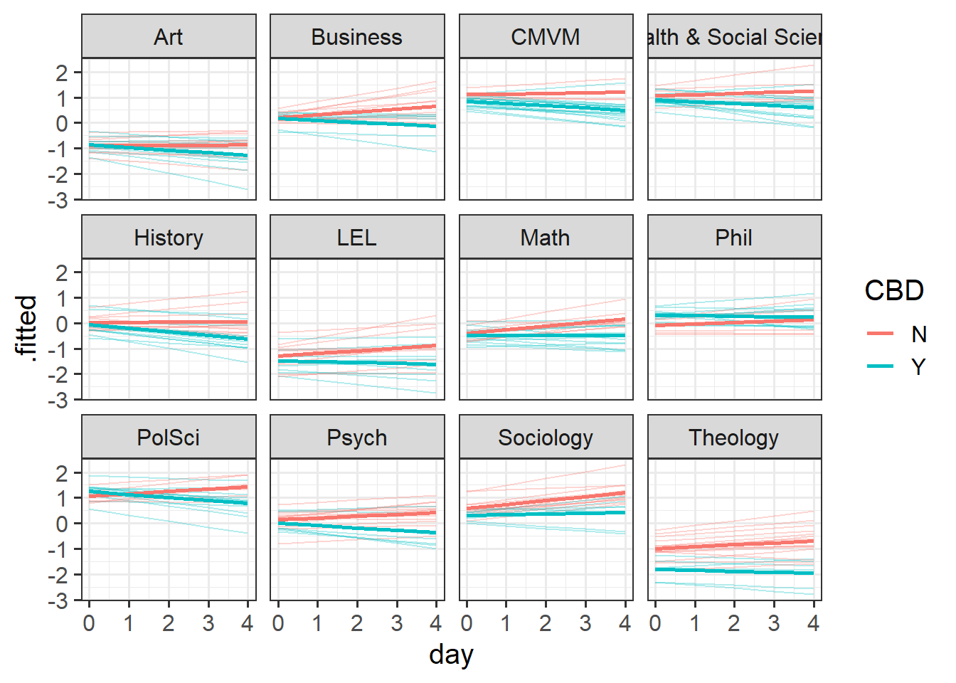

Figure 7: Plot of fitted values of the model. Individual lines for each participant, facetted by department. Thicker lines represent the department average fitted values split by CBD group

And we can see in our summary that there is a lot of by-department variation - departments vary in their baseline stress levels with a standard deviation of 0.81, and within departments, participants vary in baseline stress scores with a standard deviation of 0.38.

summary(mnest2)

...
Random effects:
 Groups   Name        Variance Std.Dev. Corr       
 dept:pid (Intercept) 0.147661 0.38427             
          day         0.012142 0.11019  -0.03      
 dept     (Intercept) 0.648410 0.80524             
          day         0.001979 0.04449  -0.18      
          CBDY        0.055388 0.23535   0.40 -0.22
 Residual             0.129765 0.36023             
Number of obs: 1200, groups:  dept:pid, 240; dept, 12
...

Examining ranef(mnest2) now gives us a list of dept:pid random effects, and then of dept random effects. We can plot them using dotplot.ranef.mer(), as seen below. From these, we can see for instance, that the effect of CBD is more negative for Theology, and Sociology and Maths have higher slopes of day. These map with the plot of fitted values we saw in Figure 7 - the department lines are going up more Math and Sociology than in other departments, and in Theology the blue CBD line is much lower relative to the red control line than in other departments.

dotplot.ranef.mer(ranef(mnest2))$dept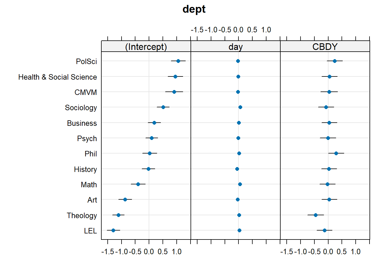

Example 3: Crossed

Forgetting about participants nested in departments, let’s return to our sample of 20 staff members from the Psychology department. In our initial study design, we had just one self report measure of stress each day for each person.
However, we might just as easily have taken more measurements. i.e. on Day 1, we could have recorded Martin’s stress levels 10 times. Furthermore, we could have used 10 different measurements of stress, rather than just a self-report measure. We could measure his cortisol levels, blood pressure, heart rate variability, give him different questionnaires, ask an informant like his son to report his stress, and so on. And we could have done the same for everybody.

stresscross <- read_csv("https://uoepsy.github.io/data/stressweek_crossed.csv")
head(stresscross)

# A tibble: 6 × 6
  dept  pid   CBD   measure          day stress
  <chr> <chr> <chr> <chr>          <dbl>  <dbl>
1 Psych Aja   N     Alpha-Amylase      1  0.269
2 Psych Aja   N     Blood Pressure     1  0.855
3 Psych Aja   N     Cortisol           1  0.278
4 Psych Aja   N     EEQ                1  0.470
5 Psych Aja   N     HRV                1 -0.404
6 Psych Aja   N     Informant          1  0.774

In this case, we can group our participants in two different ways. For each participant we have 5 datapoints for each of 10 different measures of stress. So we have 5x10 = 50 observations for each participant. But if we group them by measure instead, then we have each measure 5 times for 20 participants, so 5x20 = 100 observations of each measure. And there is no hierarchy here - the “blood pressure” measure is the same measure for Martin as it is for Dan and Aja etc. It makes sense to think of by-measure variability as not being ‘within-participants’.

This means we can choose when plotting whether to split the plots by participants, with a different line for each measure (Figure 8), or split by measure with a different line for each participant (Figure 9)

facet = participant, line = measure

Code

ggplot(stresscross, aes(x=day, y=stress, col=CBD))+
  geom_point()+
  #make a line for each measure
  geom_line(aes(group=measure))+
  facet_wrap(~pid)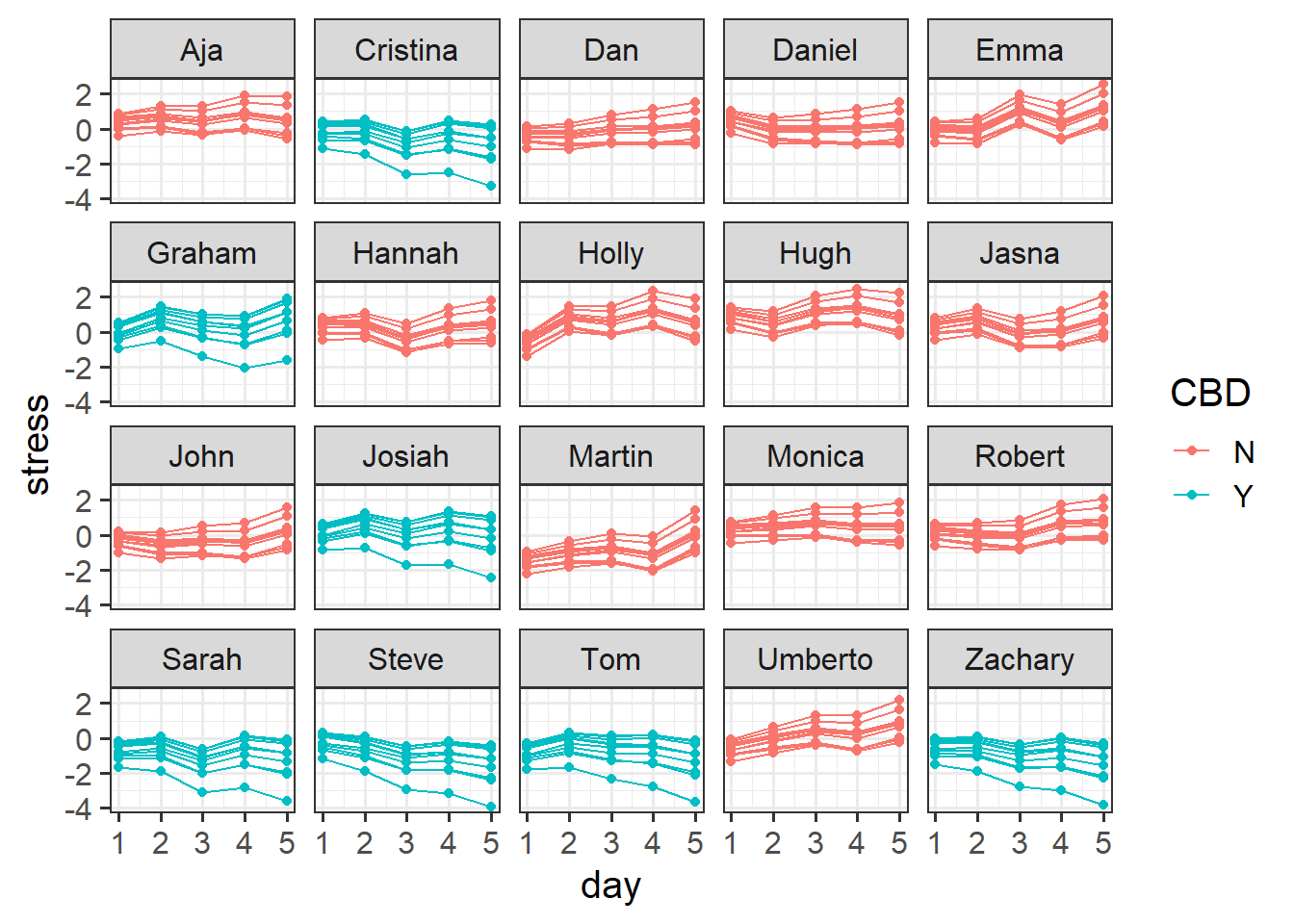

Figure 8: crossed designs with participants and measures. we can facet by participant and plot a line for each measure

facet = measure, line = participant

Code

ggplot(stresscross, aes(x=day, y=stress, col=CBD))+
  geom_point()+
  # make a line for each ppt
  geom_line(aes(group=pid))+
  facet_wrap(~measure)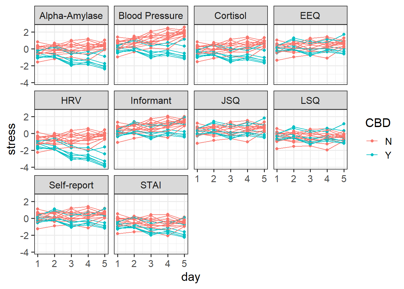

Figure 9: crossed designs with participants and measures. we can facet by measure and plot a line for each participant

We can fit a model that therefore accounts for the by-participant variation (“things vary between participants”) and the by-measure variation (“things vary between measures”).

So a model might look something like this:

# re-center 'day' so the intercept is day 1
stresscross$day <- stresscross$day-1

mcross <- lmer(stress ~ 1 + day * CBD + 
                (1 + day * CBD | measure) +
                (1 + day | pid), data = stresscross)

Note that just as with the nested example above, we can have different random slopes for measures vs those for participants, depending upon what effects can vary given the study design.

As before, removing the interaction in the random effects achieves model convergence:

mcross2 <- lmer(stress ~ 1 + day * CBD + 
                (1 + day + CBD | measure) +
                (1 + day | pid), data = stresscross)

And again we might plot our fitted values either of the ways we plotted our initial data in Figure 8 above, only with the .fitted values obtained from the augment() function:

Code

augment(mcross2) |>
  ggplot(aes(x=day, y=.fitted, col=CBD))+
    geom_point()+
    geom_line(aes(group=pid))+
    facet_wrap(~measure)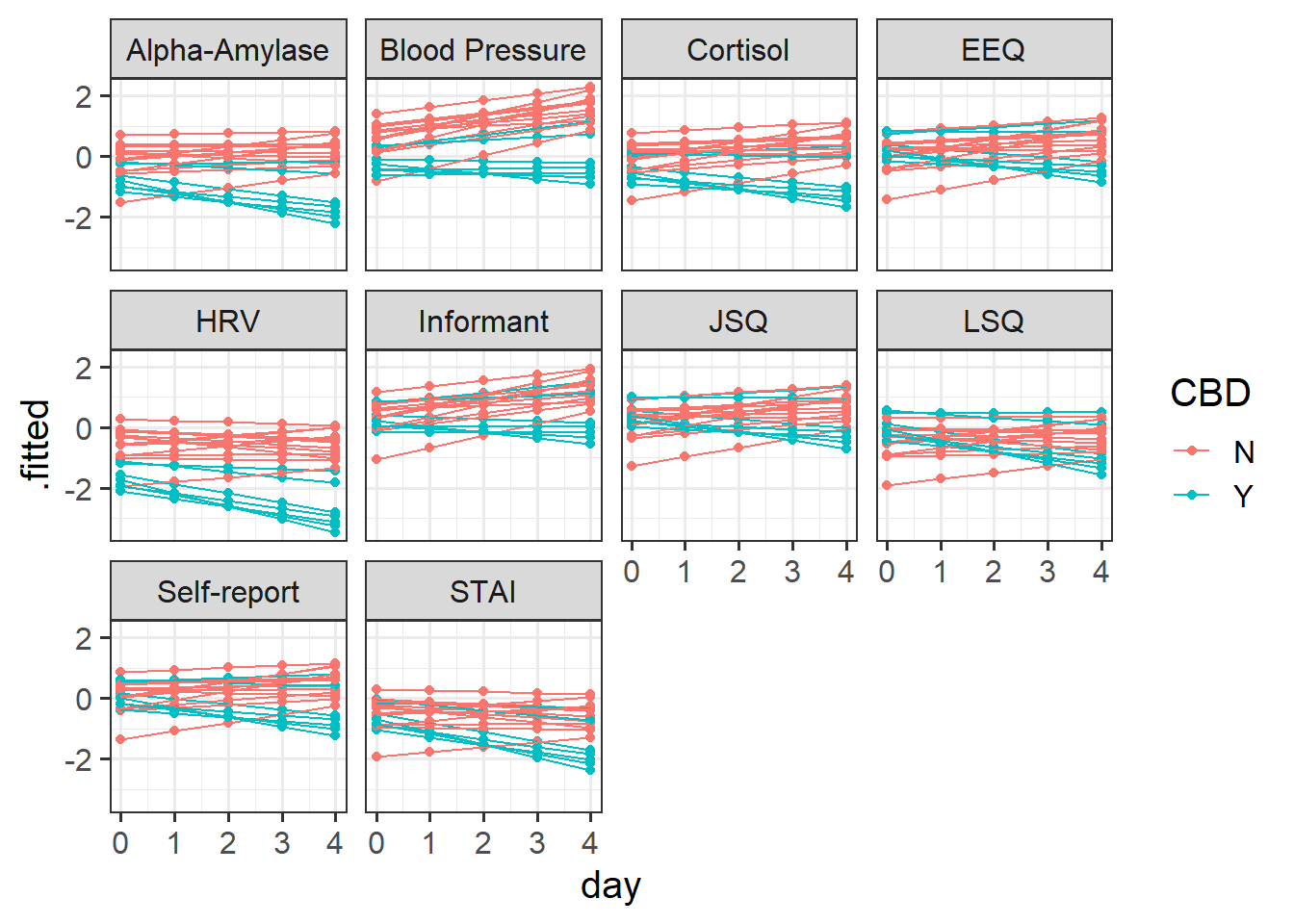

Our random effect variances show the estimated variance in different terms (the intercept, slopes of day, effect of CBD) between participants, and between measures.
From the below it is possible to see, for instance, that there is considerable variability between how measures respond to CBD (they vary in the effect of CBD on stress with a standard deviation of 0.53)

summary(mcross2)

...
Random effects:
 Groups   Name        Variance Std.Dev. Corr       
 pid      (Intercept) 0.316578 0.56265             
          day         0.014693 0.12121  -0.51      
 measure  (Intercept) 0.087111 0.29515             
          day         0.008542 0.09242   0.88      
          CBDY        0.283635 0.53257  -0.10  0.11
 Residual             0.088073 0.29677             
Number of obs: 1000, groups:  pid, 20; measure, 10
...

Again, our dotplots of random effects help to also show this picture. We can see that the measures of “blood pressure”, “alpha-amylase”, “cortisol”, and “HRV” all have more effects of CBD that are more negative. We can see this in our plot of fitted values - these measures look like CBD vs control differnce is greater than in other measures.

dotplot.ranef.mer(ranef(mcross2))$measure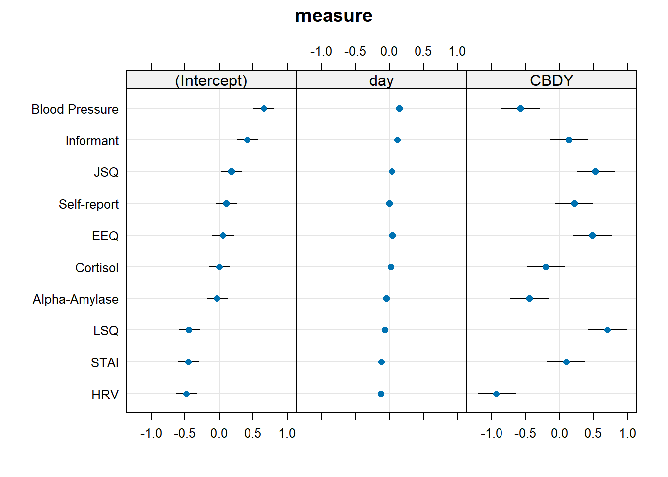

Model building

Random effect structures can get pretty complicated quite quickly. Very often it is not the random effects part that is of specific interest to us, but we wish to estimate random effects in order to more accurately partition up the variance in our outcome variable and provide better estimates of fixed effects.
It is a fine balance between fitting the most sophisticated model structure that we possibly can, and fitting a model that converges without too much simplification. Typically for many research designs, the following steps will keep you mostly on track to finding the maximal model:

lmer(outcome ~ fixed effects + (random effects | grouping structure))

1. Specify the outcome ~ fixed effects bit first.

   • The outcome variable should be clear: it is the variable we are wishing to explain/predict.
   • The fixed effects are the things we want to use to explain/predict variation in the outcome variable. These will often be the things that are of specific inferential interest, and other covariates. Just like the simple linear model.

2. If there is a grouping structure to your data, and those groups (preferably n>7 or 8) are perceived as a random sample of a wider population (the specific groups aren’t interesting to you), then consider including random intercepts (and possibly random slopes of predictors) for those groups (1 | grouping).

3. If there are multiple different grouping structures, is one nested within another? (If so, we can specify this as (1 | high_level_grouping ) + (1 | high_level_grouping:low_level_grouping). If the grouping structures are not nested, we specify them as crossed: (1 | grouping1) + (1 | grouping2).

4. If any of the things in the fixed effects vary within the groups, it might be possible to also include them as random effects.

   • as a general rule, don’t specify random effects that are not also specified as fixed effects (an exception could be specifically for model comparison, to isolate the contribution of the fixed effect).
     
   • For things that do not vary within the groups, it rarely makes sense to include them as random effects. For instance if we had a model with lmer(score ~ genetic_status + (1 + genetic_status | patient)) then we would be trying to model a process where “the effect of genetic_status on scores is different for each patient”. But if you consider an individual patient, their genetic status never changes. For patient \(i\), what is “the effect of genetic status on score”? It’s undefined. This is because genetic status only varies between patients.
   • Sometimes, things will vary within one grouping, but not within another. E.g. with patients nested within hospitals (1 | hospital) + (1 | hospital:patient), genetic_status varies between patients, but within hospitals. Therefore we could theoretically fit a random effect of genetic_status | hospital, but not one for genetic_status | patient.

5. A common approach to fitting multilevel models is to fit the most complex model that the study design allows. This means including random effects for everything that makes theoretical sense to be included. Because this “maximal model” will often not converge, we then simplify our random effect structure to obtain a convergent model.

There is no right way to simplify random effect structures - it’s about what kind of simplifications we are willing to make (a subjective decision).

Some general pointers:

• If we want to make inferences about a (within-group) fixed effect, we should ideally include it as a corresponding random effect, else we might get false positives.
  
• Complex terms like interactions (e.g. (1 + x1 * x2 | group) are often causes of non-convergence as they require more data to estimate group-level variability. This could be simplified to (1 + x1 + x2 | group)).
  
• Looking at at the random effects of a non-converging model can help point towards problematic terms. Look for random effects with little variance, or with near perfect correlation (we can alternatively remove just the correlation).
• Random effects of categorical variables often result in the model attempting to estimate a lot of variances and covariances. You could consider moving this to the right hand side (1 + catX | group) becoming (1 | group) + (1 | group:catX)

6. Obtain final model, and proceed to checking assumptions, checking influence, plotting, and eventually writing up.

model convergence

Issues of non-convergence can be caused by many things. If your model doesn’t converge, it does not necessarily mean the fit is incorrect, however it is is cause for concern, and should be addressed before using the model, else you may end up reporting inferences which do not hold.

There are lots of different things which you could do which might help your model to converge. A select few are detailed below:

• double-check the model specification and the data

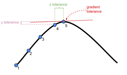
• adjust stopping (convergence) tolerances for the nonlinear optimizer, using the optCtrl argument to [g]lmerControl. (see ?convergence for convergence controls).

  • What is “tolerance”? Remember that our optimizer is the the method by which the computer finds the best fitting model, by iteratively assessing and trying to maximise the likelihood (or minimise the loss).

Figure 10: An optimizer will stop after a certain number of iterations, or when it meets a tolerance threshold

• center and scale continuous predictor variables (e.g. with scale)

• Change the optimization method (for example, here we change it to bobyqa): lmer(..., control = lmerControl(optimizer="bobyqa"))
glmer(..., control = glmerControl(optimizer="bobyqa"))

• Increase the number of optimization steps: lmer(..., control = lmerControl(optimizer="bobyqa", optCtrl=list(maxfun=50000))
glmer(..., control = glmerControl(optimizer="bobyqa", optCtrl=list(maxfun=50000))

• Use allFit() to try the fit with all available optimizers. This will of course be slow, but is considered ‘the gold standard’; “if all optimizers converge to values that are practically equivalent, then we would consider the convergence warnings to be false positives.”

• Consider simplifying your model, for example by removing random effects with the smallest variance (but be careful to not simplify more than necessary, and ensure that your write up details these changes)

singular fits

You may have noticed that some of our models over the last few weeks have been giving a warning: boundary (singular) fit: see ?isSingular.
Up to now, we’ve been largely ignoring these warnings. However, this week we’re going to look at how to deal with this issue.

boundary (singular) fit: see ?isSingular

The warning is telling us that our model has resulted in a ‘singular fit’. Singular fits often indicate that the model is ‘overfitted’ - that is, the random effects structure which we have specified is too complex to be supported by the data.

Perhaps the most intuitive advice would be remove the most complex part of the random effects structure (i.e. random slopes). This leads to a simpler model that is not over-fitted. In other words, start simplifying from the top (where the most complexity is) to the bottom (where the lowest complexity is). Additionally, when variance estimates are very low for a specific random effect term, this indicates that the model is not estimating this parameter to differ much between the levels of your grouping variable. It might, in some experimental designs, be perfectly acceptable to remove this or simply include it as a fixed effect.

A key point here is that when fitting a mixed model, we should think about how the data are generated. Asking yourself questions such as “do we have good reason to assume subjects might vary over time, or to assume that they will have different starting points (i.e., different intercepts)?” can help you in specifying your random effect structure

You can read in depth about what this means by reading the help documentation for ?isSingular. For our purposes, a relevant section is copied below:

… intercept-only models, or 2-dimensional random effects such as intercept + slope models, singularity is relatively easy to detect because it leads to random-effect variance estimates of (nearly) zero, or estimates of correlations that are (almost) exactly -1 or 1.