library(psych)
my_efa <- fa(data, nfactors = ?? , rotate = ??, fm = ??)Fitting and Comparing EFA solutions
Fitting EFA in R
The code to perform an EFA is very straightforward. It’s just one line:
The first two things we’re giving the fa() function are straightforward - we give it the dataset and we tell it how many factors we want. For rotations (rotate) and factor extraction method (fm) see Deciding on Rotation and Factor Extraction Methods.
Data
Dataset: phoneaddiction.csv
The dataset at https://uoepsy.github.io/data/phoneaddiction.csv comes from a (fake) study that is interested in developing a measure of “phone-attachment/addiction” - i.e., the idea of being overly attached to a phone.
We have a set of 10 statements (Table 1) that get at different aspects of this idea, and we asked 240 people to rate how much they agreed with each of the 10 statements on a 1-5 scale (1 = strongly disagree, 5 = strongly agree).
phdat <- read_csv("https://uoepsy.github.io/data/phoneaddiction.csv")| variable | question |
|---|---|
| item1 | I often reach for my phone even when I don't have a specific reason to use it. |
| item2 | I feel a strong urge to check my phone frequently, even during meals or social interactions. |
| item3 | I spend a large portion of my day using my phone, often for more hours than I intend. |
| item4 | My phone use has interfered with my ability to complete tasks or responsibilities at school, work, or home. |
| item5 | When I cannot use my phone (e.g., no battery or no signal), I feel anxious or uncomfortable. |
| item6 | My phone use has negatively affected my sleep schedule, such as staying up late scrolling. |
| item7 | I find it difficult to avoid checking my phone immediately upon waking up or right before bed. |
| item8 | I often check my phone even in situations where it's distracting or socially inappropriate (e.g., meetings or classes). |
| item9 | I sometimes feel that others are overly concerned about my phone use in social situations. |
| item10 | I have tried to reduce my phone usage but find it challenging to do so. |
Supposing that we are conducting EFA on our phone-addiction data, to examine what number of factors might best explain the patterns of responses to the questions.
We examine the various methods to determine a range for how many factors, and decide to consider anything from
Summary
| method | suggestion |
|---|---|
| kaiser | 3 |
| scree plot | 1 or 2/3? or 5? quite hard to tell! |
| MAP | 1 |
| parallel analysis | 2 |
Scree plot
scree(phdat)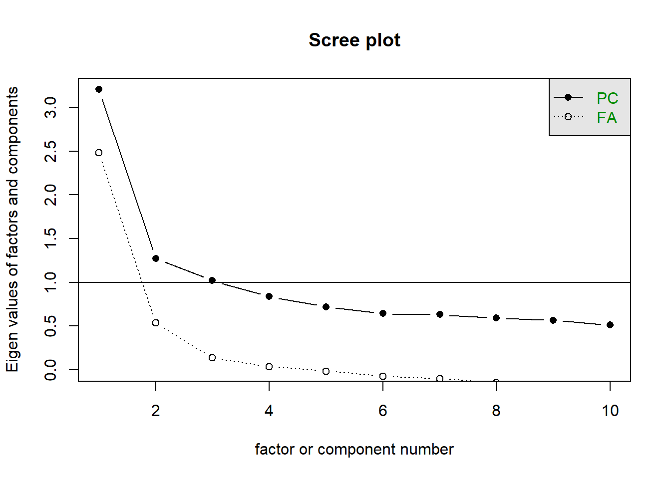
Parallel analysis
We can set fa = "both" to do the parallel analysis method for both factor extraction and principal components.
fa.parallel(phdat)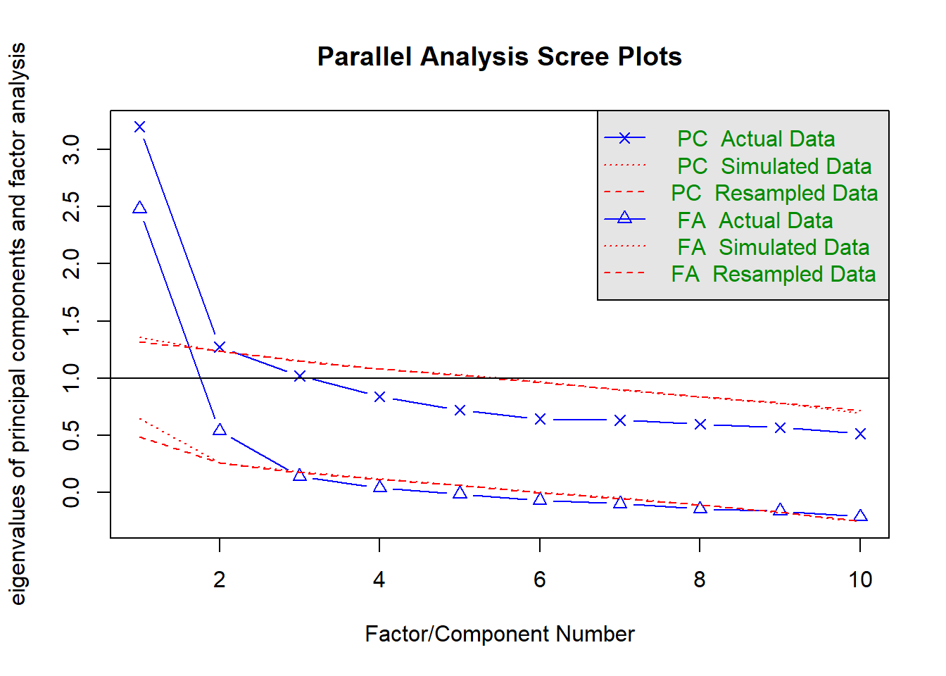
Parallel analysis suggests that the number of factors = 2 and the number of components = 1 MAP
VSS(phdat, rotate = "oblimin", plot = FALSE, fm = "ml")
Very Simple Structure
Call: vss(x = x, n = n, rotate = rotate, diagonal = diagonal, fm = fm,
    n.obs = n.obs, plot = plot, title = title, use = use, cor = cor)
VSS complexity 1 achieves a maximimum of 0.61  with  1  factors
VSS complexity 2 achieves a maximimum of 0.59  with  3  factors

The Velicer MAP achieves a minimum of 0.02  with  1  factors
BIC achieves a minimum of  -123  with  2  factors
Sample Size adjusted BIC achieves a minimum of  -40.2  with  2  factors

Statistics by number of factors
  vss1 vss2   map dof   chisq    prob sqresid  fit RMSEA  BIC SABIC complex
1 0.61 0.00 0.023  35 7.5e+01 9.9e-05     6.2 0.61 0.069 -117  -5.9     1.0
2 0.57 0.59 0.031  26 2.0e+01 8.0e-01     6.6 0.59 0.000 -123 -40.2     1.0
3 0.56 0.59 0.061  18 8.9e+00 9.6e-01     6.0 0.62 0.000  -90 -32.7     1.3
4 0.42 0.53 0.087  11 4.5e+00 9.5e-01     7.2 0.54 0.000  -56 -20.9     1.4
5 0.47 0.58 0.121   5 1.4e+00 9.3e-01     6.2 0.61 0.000  -26 -10.2     1.3
6 0.49 0.55 0.175   0 2.9e-01      NA     6.0 0.62    NA   NA    NA     1.4
7 0.37 0.41 0.279  -4 6.6e-08      NA     7.9 0.50    NA   NA    NA     1.6
8 0.34 0.39 0.493  -7 6.1e-12      NA     8.2 0.48    NA   NA    NA     1.6
   eChisq    SRMR eCRMS eBIC
1 1.0e+02 6.8e-02 0.077  -91
2 2.0e+01 3.0e-02 0.040 -123
3 8.2e+00 1.9e-02 0.031  -90
4 5.1e+00 1.5e-02 0.031  -55
5 1.1e+00 7.1e-03 0.021  -26
6 2.3e-01 3.3e-03    NA   NA
7 6.1e-08 1.7e-06    NA   NA
8 5.5e-12 1.6e-08    NA   NA
Fitting EFA models
We’re going to use an oblique rotation, because any sub-dimensions of phone-addiction are likely to be correlated (e.g., if you’re high on a ‘social FOMO driven phone-addiction’ dimension then you’re also likely to be high on a dimension that is more about being used to the physical feeling of your phone in the pocket).
We have 240 people here, and only 10 items. We will use minres to extract our factors (mainly just because it’s the default!).
We will fit a 1-, a 2-, and a 3-factor model:
ph_efa1 <- fa(phdat, nfactors = 1,
              fm = "minres")

ph_efa2 <- fa(phdat, nfactors = 2,
              fm = "minres", rotate = "oblimin")

ph_efa3 <- fa(phdat, nfactors = 3,
              fm = "minres", rotate = "oblimin")
Comparing EFA models
1 factor solution
print(ph_efa1$loadings, cutoff=.3)
Loadings:
       MR1
item1  0.555
item2  0.570
item3  0.527
item4  0.443
item5  0.518
item6  0.502
item7  0.528
item8  0.512
item9
item10 0.556

                 MR1
SS loadings    2.481
Proportion Var 0.248
2 factor solution
print(ph_efa2$loadings, cutoff=.3)
Loadings:
       MR1    MR2
item1   0.529
item2   0.556
item3   0.579
item4          0.526
item5          0.640
item6          0.509
item7   0.571
item8   0.653
item9
item10         0.680

                 MR1   MR2
SS loadings    1.684 1.438
Proportion Var 0.168 0.144
Cumulative Var 0.168 0.312ph_efa2$Phi MR1 MR2
MR1 1.000 0.577
MR2 0.577 1.0003 factor solution
print(ph_efa3$loadings, cutoff=.3)
Loadings:
       MR1    MR2    MR3
item1   0.549
item2   0.563
item3   0.606
item4          0.581
item5          0.619
item6          0.468  0.325
item7   0.552
item8   0.623
item9
item10         0.660

                 MR1   MR2   MR3
SS loadings    1.687 1.405 0.286
Proportion Var 0.169 0.141 0.029
Cumulative Var 0.169 0.309 0.338ph_efa3$Phi MR1 MR2 MR3
MR1 1.0000 0.544 0.0427
MR2 0.5444 1.000 0.1610
MR3 0.0427 0.161 1.0000
Following ‘What makes a good factor solution?’, we would probably initially conclude that the 3-factor solution is not worthwhile. It only explains 2.6% more variance (33.8 vs 31.2) than the 2-factor model, and the third factor only has one single item (item6) loaded on to it, and it’s not even that item’s primary loading.
However, in all three solutions, item9 looks like a problem item. It has smaller loadings than the other items, and doesn’t reach salience on any factor. The smaller the loading, the less well the item is targeting whatever construct the factor represents. And in none of our models does it look like the item is actually measuring anything we’re interested in.
Looking at item9, the wording is “I sometimes feel that others are overly concerned about my phone use in social situations.” This maybe represents something slightly different from just “being addicted to your phone” - it also contains a self-consciousness / feeling judged by others etc, which is something completely different. We can come up with a reasonably argument that this is perhaps capturing something separate from what the other variables are measuring.
Removing problematic items
When doing EFA, our goal will probably either be:
- to try and get a good measure that we can use in our subsequent analysis
- to develop a suitable questionnaire/measurement tool for future research
In either case, item9 isn’t proving very useful here. So we remove the variable, and then start by doing doing the entire process over again!
phdatB <- phdat |> select(-item9)Begin again…
Once we remove item9, we must go back to determining a range for the number of factors:
| method | suggestion |
|---|---|
| kaiser | 2 |
| scree plot | 1 or 2 |
| MAP | 1 |
| parallel analysis | 1 or 2 |
And then fitting these to the new, reduced data. We are no longer examining the 3-factor model because that no longer looked as feasible given the methods above.
ph_efaB1 <- fa(phdatB, nfactors = 1,
              fm = "minres")

ph_efaB2 <- fa(phdatB, nfactors = 2,
              fm = "minres", rotate = "oblimin")
Comparing EFA models
1 factor solution
print(ph_efaB1$loadings, cutoff=.3)
Loadings:
       MR1
item1  0.558
item2  0.570
item3  0.526
item4  0.443
item5  0.516
item6  0.502
item7  0.529
item8  0.513
item10 0.555

                 MR1
SS loadings    2.478
Proportion Var 0.275
2 factor solution
print(ph_efaB2$loadings, cutoff=.3)
Loadings:
       MR1    MR2
item1   0.517
item2   0.553
item3   0.585
item4          0.529
item5          0.634
item6          0.517
item7   0.567
item8   0.657
item10         0.677

                 MR1   MR2
SS loadings    1.673 1.430
Proportion Var 0.186 0.159
Cumulative Var 0.186 0.345ph_efa2$Phi MR1 MR2
MR1 1.000 0.577
MR2 0.577 1.000Comparing these two solutions (1-factor and 2-factor), we can see that the 2-factor model explains 7% more variance (34.5 vs 27.5). Both solutions have factors have >3 items with salient loadings, and there are no cross-loadings or anything looking too problematic.
Numerically, both look fine! And the increase in variance explained is ~7%, which isn’t nothing, but it doesn’t feel like a huge amount either.
This is a good example of where the theoretical coherence of the two models is going to come to the fore.
In the 1-factor solution, we are saying that there is just one underlying thing, and that thing is “phone-attachment/addiction”.
In the 2-factor solution, we are saying that we need 2 related things (with a correlation of 0.58) to explain how people respond to the questions.
Those two things are defined by how they relate to the different items. Given the item wordings below, we might try to define Factor 1 as “frequency of use” and Factor 2 as “impact on life”.
Are these distinct enough for you? Personally I would say maybe not - some of the wordings of items in Factor 1 are still related to “impact on life” (i.e., “often for more hours than I intend”?)
This is ultimately a judgement call, and will require more background reading into the literature on addiction/phone-addiction etc. A really strong investigation could be paired with some qualitative interviews with people ‘thinking-aloud’ through their response process for the set of items.
Factor 1
| variable | question |
|---|---|
| item1 | I often reach for my phone even when I don't have a specific reason to use it. |
| item2 | I feel a strong urge to check my phone frequently, even during meals or social interactions. |
| item3 | I spend a large portion of my day using my phone, often for more hours than I intend. |
| item7 | I find it difficult to avoid checking my phone immediately upon waking up or right before bed. |
| item8 | I often check my phone even in situations where it's distracting or socially inappropriate (e.g., meetings or classes). |
Factor 2
| variable | question |
|---|---|
| item4 | My phone use has interfered with my ability to complete tasks or responsibilities at school, work, or home. |
| item5 | When I cannot use my phone (e.g., no battery or no signal), I feel anxious or uncomfortable. |
| item6 | My phone use has negatively affected my sleep schedule, such as staying up late scrolling. |
| item10 | I have tried to reduce my phone usage but find it challenging to do so. |