Check assumptions

Example: University job satisfaction

Let’s suppose we are studying employee job satisfaction at the university, and we want to estimate the association between pay-scale and job satisfaction, controlling for the NSS rating of departments.

We have 399 employees from 25 different departments, and we got them to fill in a job satisfaction questionnaire, and got information on what their payscale was. We have also taken information from the National Student Survey on the level of student satisfaction for each department.

Each datapoint here represents an individual employee, and these employees are grouped into departments.

variable	description
NSSrating	National Student Satisfaction rating for the department
dept	Department name
payscale	Pay scale of employee
jobsat	Job satisfaction of employee
jobsat_binary	Binary question of whether the employee considered themselves to be satisfied with their work (1) or not (0)

jobsat <- read_csv("https://uoepsy.github.io/data/msmr_nssjobsat.csv")

Here’s the maximal model for this data:

jobsat_mod <- lmer(
  jobsat ~ payscale + NSSrating + (1 + payscale | dept), 
  data = jobsat
)

We are predicting employee’s job satisfaction as a function of their pay scale and the department’s NSS rating. We’re also including by-department adjustments to the fixed intercept and to the slope over payscale.

Linearity of association

It’s standard practice in Psychology to accept that this assumption is met. Why? Because if we want to use the linear modelling machinery at all (which we do, because it’s the standard in the field), we must assume that the associations we want to model are sufficiently linear.

Independence of errors

If you are using an appropriate random effect structure in your model (see Identify possible random effects), then you can consider the assumption of independence of errors to be met.

Normal distribution of errors

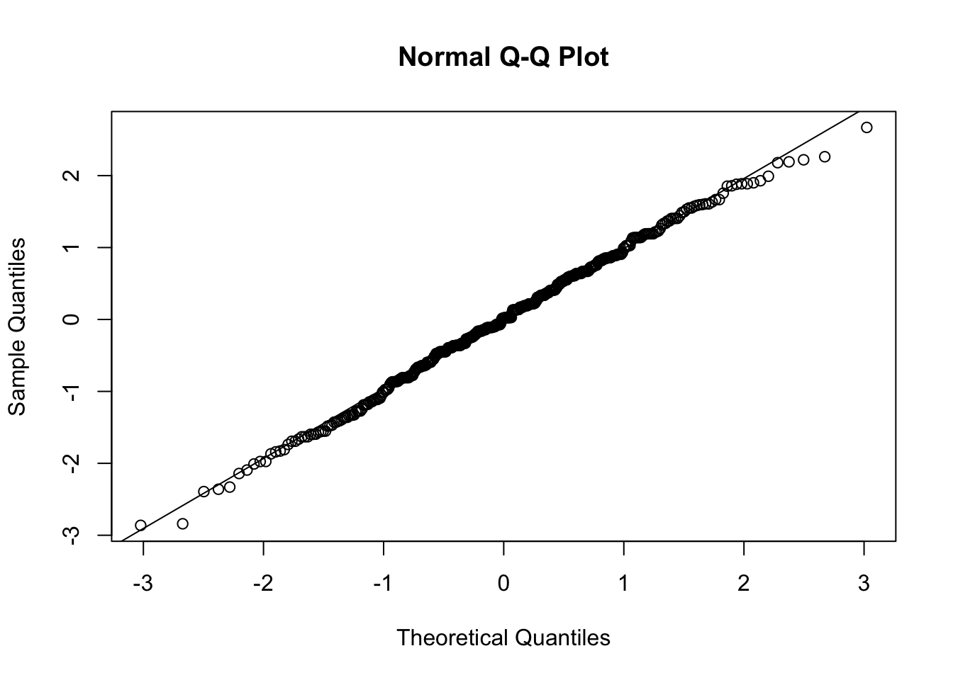
As in DAPR2, we can use a Q-Q plot to visually inspect the normality of the model’s residuals. We want the sample quantiles (the residuals of our model, the circular points) to closely match the theoretical quantiles (an ideal normal distribution, the diagonal line from bottom left to top right).

qqnorm(resid(jobsat_mod))
qqline(resid(jobsat_mod))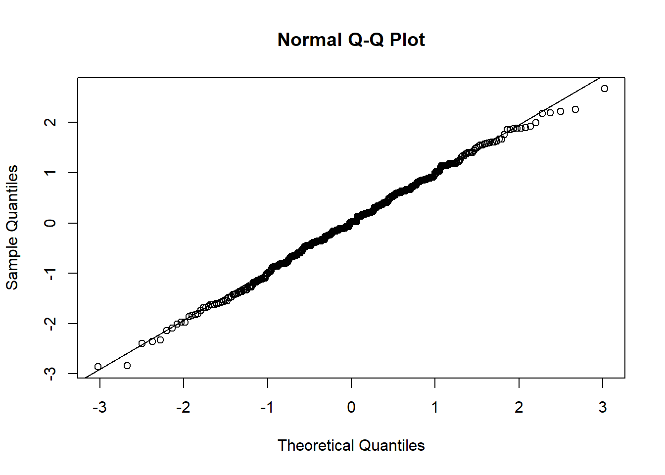

A pretty good match! No cause for concern.

Normal distribution of random effects

We extract the model’s random effects for dept using the ranef() function, and we get the by-department intercept adjustments by selecting the first column:

ranef(jobsat_mod)$dept[,1]

 [1]  0.5791  0.2438  0.1454  0.4805  0.2942 -0.5282 -0.2786 -0.2909  0.0169
[10] -0.2279 -0.0305 -0.2934 -0.9244  0.1112  0.1437 -0.7285  0.0128  0.1980
[19]  0.0104  0.3166 -0.0347  0.2181  0.3473 -0.5233  0.7426

Then we use this data in the Q-Q plot to check the normality of the model’s random intercepts:

qqnorm(ranef(jobsat_mod)$dept[,1]) 
qqline(ranef(jobsat_mod)$dept[,1])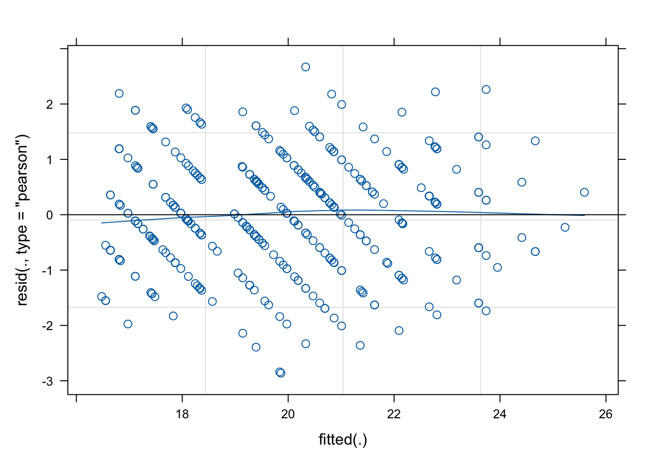

The by-department intercept adjustments match the diagonal line pretty well. Not a cause for concern.

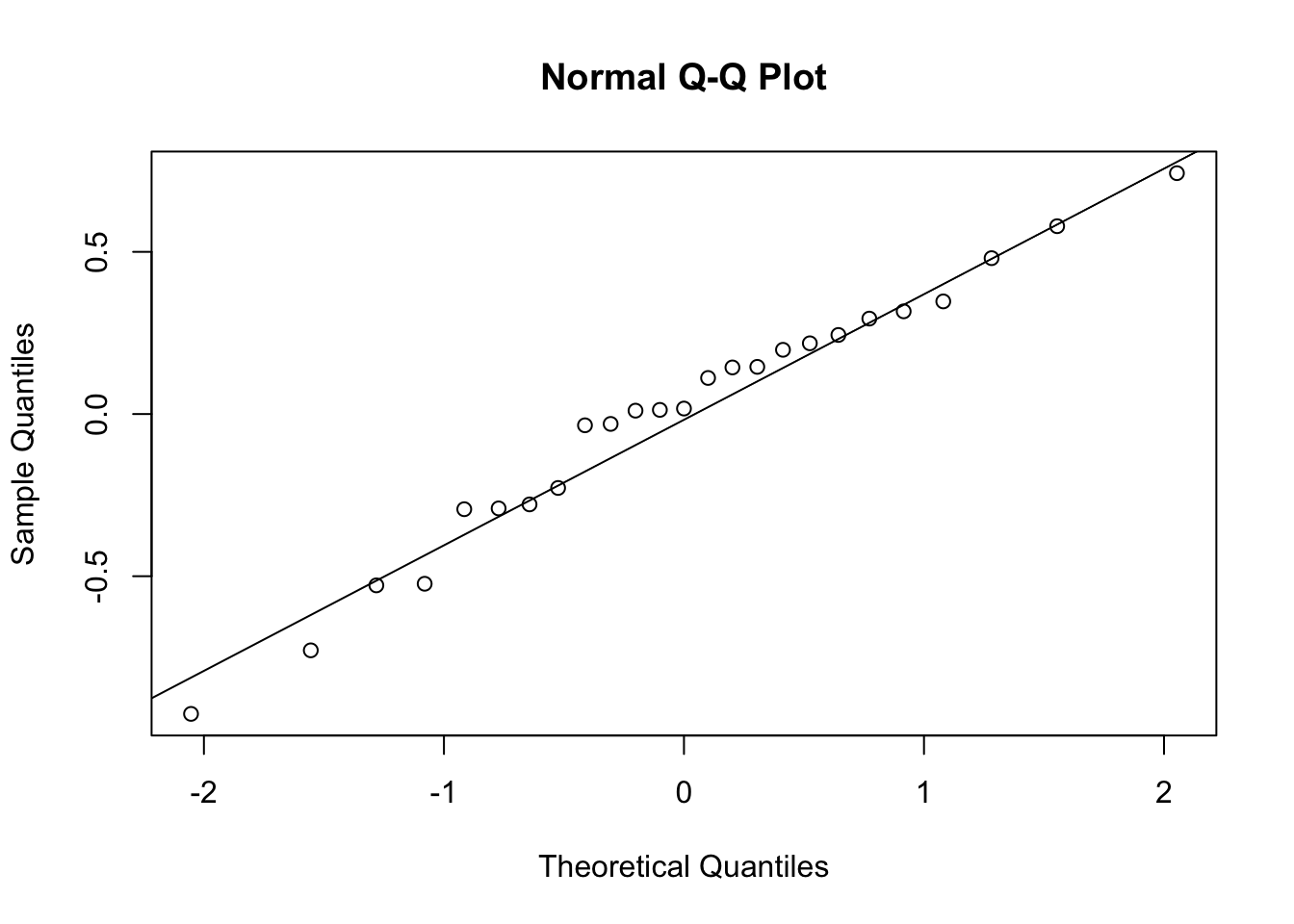
To get the random slopes, we can grab the second column from the ranef() output and make the same Q-Q plot:

qqnorm(ranef(jobsat_mod)$dept[,2]) 
qqline(ranef(jobsat_mod)$dept[,2])

The by-department adjustments to the slope over payscale also match the diagonal line pretty well. No cause for concern here either.

Equal variance of errors

As in DAPR2, we can use a residuals-vs-fitted plot to visually inspect the variance of the model’s residuals. We want the vertical spread of the residuals to be approximately the same everywhere.

plot(jobsat_mod, 
     type=c(
       "p",      # includes points representing Pearson residuals
       "smooth"  # includes smoothed line representing mean of residuals
       )
    )

The vertical spread tapers off a little bit toward higher fitted values, but it’s not too dramatic. Overall it’s a reasonably even cloud of data points, so no cause for concern.

(Why are the points appearing in diagonal lines? Because the observed outcome values are whole numbers only, with no decimal values to fill in the gaps in between.)