Getting PCA Scores

Data

Dataset: physfunc.csv

These data contain measurements on 220 individuals on various measures of physical functioning:

• Mobility: 6-Minute Walk Test (distance in metres walked in 6 minutes).
• Balance: Single-Leg Stance Test (time in seconds standing on one leg).
• Endurance: Stair Climb Test (time in seconds taken to climb a set number of stairs).
• Flexibility: Sit and Reach Test (distance in cm reached beyond the feet while seated).
• Strength: Grip Strength Test (measured in kilograms using a dynamometer).
• Fine Motor Skills: Nine-Hole Peg Test (time in seconds to place and remove pegs from a board).
• Respiratory Function: Forced Expiratory Volume in 1 Second (FEV1) (measured in Liters per second using a spirometer).

Dataset: https://uoepsy.github.io/data/physfunc.csv

physfunc <- read_csv("https://uoepsy.github.io/data/physfunc.csv")
head(physfunc)

# A tibble: 6 × 8
  mobility balance endurance flexibility strength coordination fine_motor
     <dbl>   <dbl>     <dbl>       <dbl>    <dbl>        <dbl>      <dbl>
1      587    23.7      13.1          11       43         1.62       20.8
2      594    23.8      12.9           9       33         1.56       20.8
3      554    29.1      14.3          12       50         1.69       22  
4      525    17.9      16.6           8       20         1.62       20.1
5      541    17.5      20.0           9       43         1.45       20.6
6      540    21.7      16.2          10       40         1.51       20.0
# ℹ 1 more variable: respiratory <dbl>

Doing PCA

Using principal() from the {psych} package, with 8 observed variables, we are working in 8 observed dimensions (our measured variables). These variables are all correlated, and PCA re-expresses the information onto un-correlated (i.e. perpendicular) dimensions.

With 8 measured variables, we get out 8 orthogonal dimensions, which here we call “principal components”.
In the principal() function, we can set nfactors = 8 to extract 8 dimensions. If we specified a lower number, e.g., nfactors = 6, it would simply not show the 7th and 8th components.

Setting rotate = "none" ensures that these new dimensions are orthogonal to one another.

library(psych)
fullpca <- principal(physfunc, nfactors = 8, 
                     rotate = "none")

The output of our PCA gives us two sections:

• “loadings”: correlations between each new dimension and the original dimensions
• “SSloadings”: total variance captured by each new dimension.

Along with various other methods, we can use the latter to decide how many components to keep.

the output

fullpca

Principal Components Analysis
Call: principal(r = physfunc, nfactors = 8, rotate = "none")
Standardized loadings (pattern matrix) based upon correlation matrix
               PC1   PC2   PC3   PC4   PC5   PC6   PC7   PC8 h2       u2 com
mobility      0.89  0.04 -0.11  0.35 -0.21  0.01 -0.18  0.01  1  0.0e+00 1.6
balance       0.90  0.04  0.03 -0.33  0.22  0.10 -0.18  0.01  1  1.1e-15 1.5
endurance    -0.12  0.95  0.01  0.01 -0.07  0.27  0.05  0.00  1 -1.3e-15 1.2
flexibility   0.74  0.08  0.58  0.27  0.19 -0.01  0.06 -0.02  1  1.6e-15 2.4
strength      0.83  0.07  0.39 -0.27 -0.26 -0.08  0.09  0.02  1  1.3e-15 1.9
coordination  0.88 -0.01 -0.40  0.10  0.17  0.00  0.16  0.04  1  1.1e-16 1.6
fine_motor    0.92  0.01 -0.36 -0.09 -0.10 -0.02  0.06 -0.05  1  7.8e-16 1.4
respiratory  -0.07  0.95 -0.08 -0.02  0.08 -0.27 -0.05  0.00  1 -1.1e-15 1.2

                       PC1  PC2  PC3  PC4  PC5  PC6  PC7  PC8
SS loadings           4.46 1.82 0.80 0.39 0.24 0.16 0.11 0.01
Proportion Var        0.56 0.23 0.10 0.05 0.03 0.02 0.01 0.00
Cumulative Var        0.56 0.79 0.89 0.93 0.96 0.99 1.00 1.00
Proportion Explained  0.56 0.23 0.10 0.05 0.03 0.02 0.01 0.00
Cumulative Proportion 0.56 0.79 0.89 0.93 0.96 0.99 1.00 1.00

Mean item complexity =  1.6
Test of the hypothesis that 8 components are sufficient.

The root mean square of the residuals (RMSR) is  0 
 with the empirical chi square  0  with prob <  NA 

Fit based upon off diagonal values = 1

How many components should we keep?

Using methods detailed in Deciding on the Number of Components, we make a decision on how many components to keep, and therefore how many to discard.

For this dataset, we might end up with these recommendations:

method	suggestion
scree plot	1 or 2
MAP	1
parallel analysis	2
keeping 50% variance	1
keeping 75% variance	2
keeping 80% variance	3
keeping 90% variance	4

See for yourself

Variance captured
We can see the cumulative proportion of variance being captured in the bottom row here:

fullpca$Vaccounted

                        PC1   PC2    PC3    PC4    PC5    PC6    PC7      PC8
SS loadings           4.462 1.823 0.7974 0.3943 0.2423 0.1649 0.1104 0.005247
Proportion Var        0.558 0.228 0.0997 0.0493 0.0303 0.0206 0.0138 0.000656
Cumulative Var        0.558 0.786 0.8854 0.9346 0.9649 0.9855 0.9993 1.000000
Proportion Explained  0.558 0.228 0.0997 0.0493 0.0303 0.0206 0.0138 0.000656
Cumulative Proportion 0.558 0.786 0.8854 0.9346 0.9649 0.9855 0.9993 1.000000

The first component captures 55.8%
The first two components capture 78.6% The first three components capture 88.5%
… … All eight components capture 100%

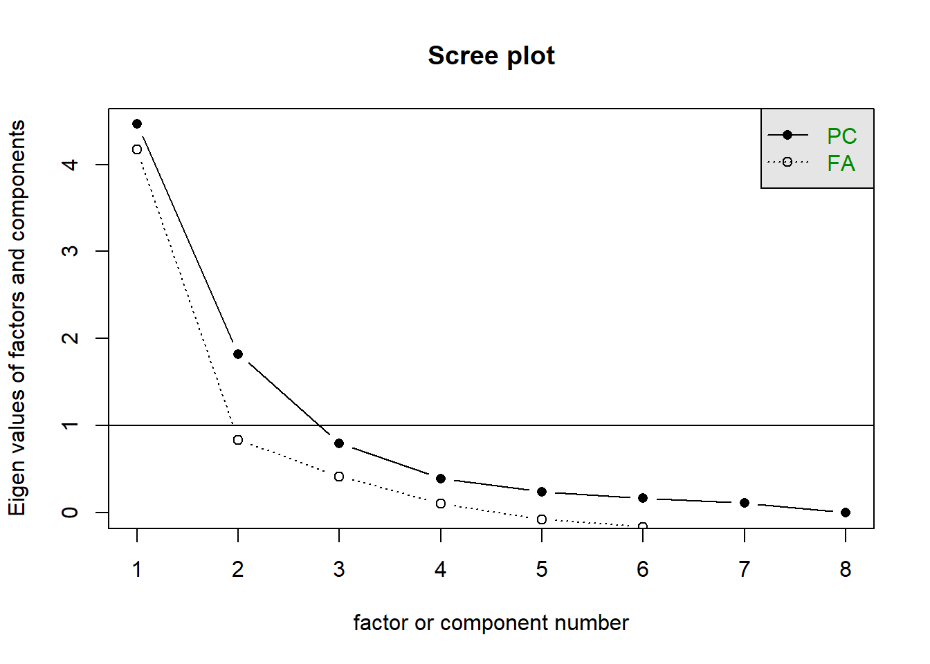
Scree Plot

The screeplot shows a possible kink at either the second or third, indicating that we keep either 1 or 2.

cor(physfunc) |>
  scree()

Minimum Average Partial (MAP)
There’s a lot of output from VSS() and we’re only really interested in the map values, so let’s pull those out.
We can see that the first value is lowest, suggesting 1 component:

VSS(physfunc, n = 8, 
    rotate = "none", plot = FALSE)$map

[1] 0.137 0.152 0.188 0.279 0.426 0.835 1.000    NA

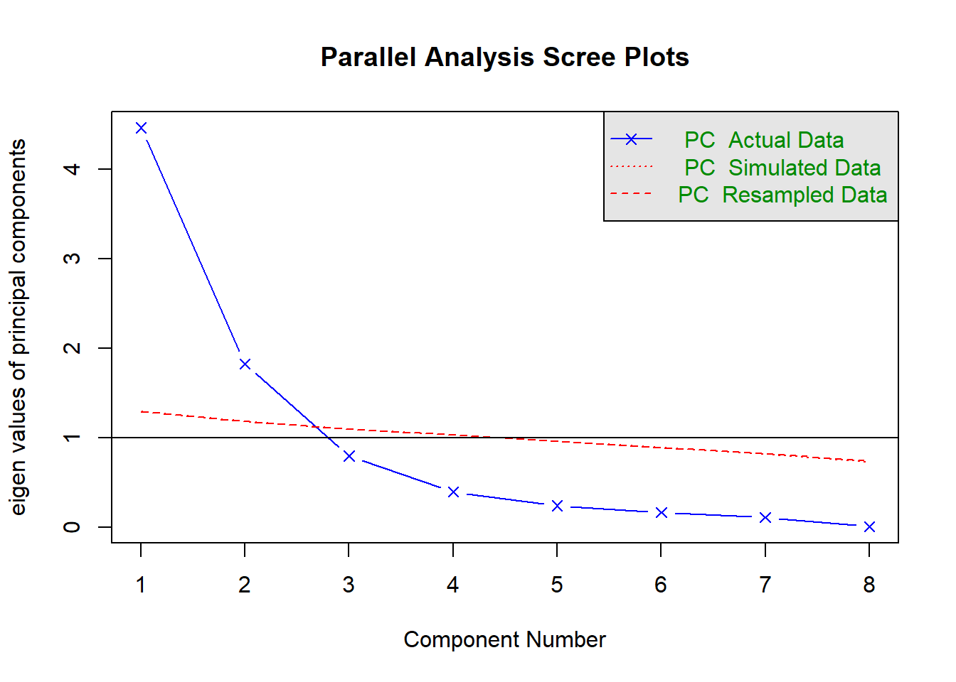
Parallel Analysis
This approach suggests 2 components:

fa.parallel(physfunc,
            fa = "pc",
            n.iter = 500)

Parallel analysis suggests that the number of factors =  NA  and the number of components =  2 

Let’s suppose that we decide to retain two components, capturing 79% of the total variance:

pca_2dim <- principal(physfunc, 
                      nfactors = 2, rotate = "none")

extracting scores

When it comes to using the principal components in some subsequent analysis, we need to access the “scores”.

These are already stored in the PCA, in the $scores slot:

pca_2dim$scores

        PC1      PC2
[1,]  0.84411 -0.91828
[2,]  0.30184 -0.73377
[3,]  1.40557 -0.10588
[4,] -0.62169 -0.08713
[5,] -0.05582  1.94701
[6,]  0.23296  0.25940
..      ...      ...
..      ...      ...

So we can add these scores to our data:

physfunc$pc1 <- pca_2dim$scores[,1]
physfunc$pc2 <- pca_2dim$scores[,2]

And then go and use those in some subsequent analysis instead of our original 8 variables!