PCA
Introducing PCA
Principal Components Analysis (PCA) is a method of dimension reduction that decomposes a \(p \times p\) covariance or correlation matrix into a new set of \(p\) “orthogonal” (uncorrelated to one another) dimensions. These dimensions sequentially capture as much of the variance in the data as possible.
In the simple example where we have 3 measured variables, and this can be illustrated in the 3D scatterplot as in Figure 1, PCA provides us with new dimensions that capture the variability in the data (these are represented by the coloured axes in the plot).
When we do PCA, we get out two key things about our new dimensions:
- magnitude: how much variability is captured by the new dimension
- direction: how the new dimension relates to the original measured variables
Strictly speaking, PCA is not really an “explanatory” tool. It simply combines variables to preserve variance. This means we are less interested in the directions of the dimensions, and mainly focussed on how much variance they capture.
What we then do is simply decide how many of these new dimensions we want to keep (and therefore, how much variance in the data we are willing to sacrifice).
Rabbit Hole - eigen decomposition
Behind the scenes, this is achieved using “eigen decomposition” which is a fairly complex calculation performed on the correlation matrix.1
The main thing to takeaway from this is that for each of these new dimensions we get two things (“eigenvalues” and “eigenvectors”) that are essentially:
- magnitude (“eigenvalues”): how long the new dimension is
- direction (“eigenvectors”): how the new dimension relates to the original dimensions.

Some of the maths behind it
A correlation matrix is a square matrix (i.e. same number of columns as rows), and it is symmetric on the diagonals. Furthermore, the diagonal values themselves are all 1 (the correlation of a variable with itself is 1).
So we might see a correlation matrix (lets call it \(\mathbf{R}\)) that looks like this:
\[ \begin{equation*} \mathbf{R} = \begin{bmatrix} 1.00, 0.72, 0.63, 0.54, 0.45, 0.36 \\ 0.72, 1.00, 0.56, 0.48, 0.40, 0.32 \\ 0.63, 0.56, 1.00, 0.42, 0.35, 0.28 \\ 0.54, 0.48, 0.42, 1.00, 0.30, 0.24 \\ 0.45, 0.40, 0.35, 0.30, 1.00, 0.20 \\ 0.36, 0.32, 0.28, 0.24, 0.20, 1.00 \\ \end{bmatrix} \end{equation*} \]
One way in which we can create a symmetric square matrix is to take the product of some vector \(\mathbf{f}\) with \(\mathbf{f'}\) (\(\mathbf{f}\) “transposed”). This is just how you might “square” a vector. To multiply two vectors you take each entry of the first and multiply it with each entry of the second.
For instance:
\[
\begin{equation*}
\mathbf{f} =
\begin{bmatrix}
0.88 \\
0.83 \\
0.77 \\
0.69 \\
0.60 \\
0.50 \\
\end{bmatrix}
\qquad
\mathbf{f} \mathbf{f'} =
\begin{bmatrix}
0.88 \\
0.83 \\
0.77 \\
0.69 \\
0.60 \\
0.50 \\
\end{bmatrix}
\begin{bmatrix}
0.88, 0.83, 0.77, 0.69, 0.60, 0.50 \\
\end{bmatrix}
\qquad = \qquad
\begin{bmatrix}
0.78, 0.74, 0.68, 0.61, 0.53, 0.44 \\
0.74, 0.69, 0.64, 0.58, 0.50, 0.42 \\
0.68, 0.64, 0.59, 0.53, 0.47, 0.39 \\
0.61, 0.58, 0.53, 0.48, 0.42, 0.35 \\
0.53, 0.50, 0.47, 0.42, 0.37, 0.30 \\
0.44, 0.42, 0.39, 0.35, 0.30, 0.25 \\
\end{bmatrix}
\end{equation*}
\]
Note that I’ve chosen values for \(\mathbf{f}\) that get pretty close to re-creating \(\mathbf{R}\) (clever me!). I can get even closer if I take this and add to it the product of another vector:
\[ \begin{align} \begin{bmatrix} 0.78, 0.74, 0.68, 0.61, 0.53, 0.44 \\ 0.74, 0.69, 0.64, 0.58, 0.50, 0.42 \\ 0.68, 0.64, 0.59, 0.53, 0.47, 0.39 \\ 0.61, 0.58, 0.53, 0.48, 0.42, 0.35 \\ 0.53, 0.50, 0.47, 0.42, 0.37, 0.30 \\ 0.44, 0.42, 0.39, 0.35, 0.30, 0.25 \\ \end{bmatrix} &+ \begin{bmatrix} 0.06 \\ 0.07 \\ 0.09 \\ 0.13 \\ 0.27 \\ -0.85 \\ \end{bmatrix} \begin{bmatrix} 0.06, 0.07, 0.09, 0.13, 0.27, -0.85 \\ \end{bmatrix} \qquad = \qquad \\ \quad \\ \quad \\ \begin{bmatrix} 0.78, 0.74, 0.68, 0.61, 0.53, 0.44 \\ 0.74, 0.69, 0.64, 0.58, 0.50, 0.42 \\ 0.68, 0.64, 0.59, 0.53, 0.47, 0.39 \\ 0.61, 0.58, 0.53, 0.48, 0.42, 0.35 \\ 0.53, 0.50, 0.47, 0.42, 0.37, 0.30 \\ 0.44, 0.42, 0.39, 0.35, 0.30, 0.25 \\ \end{bmatrix} &+ \begin{bmatrix} 0.00, 0.00, 0.00, 0.01, 0.02, 0.05 \\ 0.00, 0.00, 0.01, 0.01, 0.02, 0.06 \\ 0.00, 0.01, 0.01, 0.01, 0.02, 0.07 \\ 0.01, 0.01, 0.01, 0.02, 0.03, 0.11 \\ 0.02, 0.02, 0.02, 0.03, 0.07, 0.23 \\ 0.05, 0.06, 0.07, 0.11, 0.23, 0.72 \\ \end{bmatrix} \qquad = \qquad \begin{bmatrix} 0.78, 0.74, 0.68, 0.62, 0.55, 0.40 \\ 0.74, 0.70, 0.65, 0.59, 0.52, 0.36 \\ 0.68, 0.65, 0.60, 0.55, 0.49, 0.31 \\ 0.62, 0.59, 0.55, 0.50, 0.45, 0.24 \\ 0.55, 0.52, 0.49, 0.45, 0.44, 0.07 \\ 0.40, 0.36, 0.31, 0.24, 0.07, 0.97 \\ \end{bmatrix} \end{align} \]
I haven’t just chosen a random additional vector here, I’ve chosen one that is “orthogonal” to the first vector (this gets a little complicated and trigonometry-related, but click here for an explanation of why the dot product of orthogonal vectors is equal to zero).
\[ \begin{align} \begin{bmatrix} 0.88 \\ 0.83 \\ 0.77 \\ 0.69 \\ 0.60 \\ 0.50 \\ \end{bmatrix} \cdot \begin{bmatrix} 0.06 \\ 0.07 \\ 0.09 \\ 0.13 \\ 0.27 \\ -0.85 \\ \end{bmatrix} = 0 \end{align} \]
In essence eigen decomposition is about finding a set of vectors that can, together, express our correlation matrix \(\mathbf{R}\).
For an \(n \times n\) correlation matrix \(\mathbf{R}\), there is a set of \(n\) eigenvectors \(x_i\) that solve the equation \[
\mathbf{x_i R} = \lambda_i \mathbf{x_i}
\] Where the vector multiplied by the correlation matrix is equal to some eigenvalue \(\lambda_i\) multiplied by that vector.
We can write this without subscript \(i\) as: \[
\begin{align}
& \mathbf{R X} = \mathbf{X \lambda} \\
& \text{where:} \\
& \mathbf{R} = \text{correlation matrix} \\
& \mathbf{X} = \text{matrix of eigenvectors} \\
& \mathbf{\lambda} = \text{vector of eigenvalues}
\end{align}
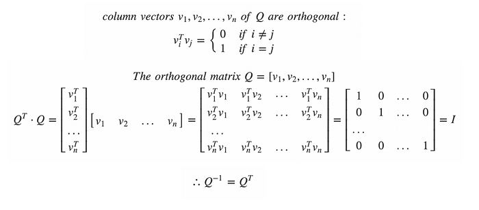
\] these vectors that make up \(\mathbf{X}\) are orthogonal (\(\mathbf{XX' = I}\)), which means that \(\mathbf{R = X \lambda X'}\)
For some demonstration in R, let’s create a correlation matrix
# lets create a correlation matrix, as f f'
f <- seq(.9,.4,-.1)
R <- f %*% t(f)
#give rownames and colnames
rownames(R)<-colnames(R)<-paste0("V",seq(1:6))
#constrain diagonals to equal 1
diag(R)<-1
# here's our correlation matrix!
R
V1 V2 V3 V4 V5 V6
V1 1.00 0.72 0.63 0.54 0.45 0.36
V2 0.72 1.00 0.56 0.48 0.40 0.32
V3 0.63 0.56 1.00 0.42 0.35 0.28
V4 0.54 0.48 0.42 1.00 0.30 0.24
V5 0.45 0.40 0.35 0.30 1.00 0.20
V6 0.36 0.32 0.28 0.24 0.20 1.00The actual solving of the eigen decomposition is too much for me, but luckily the function eigen() does it for us!
# do eigen decomposition
e <- eigen(R)
print(e, digits=2)
eigen() decomposition
$values
[1] 3.16 0.82 0.72 0.59 0.44 0.26
$vectors
[,1] [,2] [,3] [,4] [,5] [,6]
[1,] -0.50 -0.061 0.092 0.14 0.238 0.816
[2,] -0.47 -0.074 0.121 0.21 0.657 -0.533
[3,] -0.43 -0.096 0.182 0.53 -0.675 -0.184
[4,] -0.39 -0.142 0.414 -0.78 -0.201 -0.104
[5,] -0.34 -0.299 -0.860 -0.20 -0.108 -0.067
[6,] -0.28 0.934 -0.178 -0.10 -0.067 -0.045It returns eigenvalues and corresponding eigenvectors.
The eigenvectors are orthogonal (\(\mathbf{XX' = I}\)):
round(e$vectors %*% t(e$vectors),2) [,1] [,2] [,3] [,4] [,5] [,6]
[1,] 1 0 0 0 0 0
[2,] 0 1 0 0 0 0
[3,] 0 0 1 0 0 0
[4,] 0 0 0 1 0 0
[5,] 0 0 0 0 1 0
[6,] 0 0 0 0 0 1The eigenvectors represent the direction of the vectors, and the eigenvalues represent magnitude (i.e., how much variance of \(\mathbf{R}\) they capture).
Our Principal Components \(\mathbf{P}\) are the eigenvectors scaled by the square root of the eigenvalues:
# eigenvectors
# e$vectors
# scaled by sqrt of eigenvalues
# diag(sqrt(e$values))

P <- e$vectors %*% diag(sqrt(e$values))
P
[,1] [,2] [,3] [,4] [,5] [,6]
[1,] -0.883 -0.0554 0.0782 0.1070 0.1584 0.4174
[2,] -0.833 -0.0673 0.1025 0.1648 0.4361 -0.2727
[3,] -0.770 -0.0873 0.1542 0.4077 -0.4483 -0.0943
[4,] -0.694 -0.1284 0.3512 -0.5987 -0.1332 -0.0530
[5,] -0.604 -0.2712 -0.7293 -0.1514 -0.0715 -0.0342
[6,] -0.502 0.8464 -0.1513 -0.0771 -0.0443 -0.0231$$ R = PP’
X
$$
And with all of them, we can perfectly reproduce our correlation matrix: \(\mathbf{R = PP'}\).
P %*% t(P) [,1] [,2] [,3] [,4] [,5] [,6]
[1,] 1.00 0.72 0.63 0.54 0.45 0.36
[2,] 0.72 1.00 0.56 0.48 0.40 0.32
[3,] 0.63 0.56 1.00 0.42 0.35 0.28
[4,] 0.54 0.48 0.42 1.00 0.30 0.24
[5,] 0.45 0.40 0.35 0.30 1.00 0.20
[6,] 0.36 0.32 0.28 0.24 0.20 1.00But we don’t want to keep all of them, because then we are not reducing anything. So we might choose to keep, e.g., just one.
When “doing PCA” with the principal() function, we retain only one component with nfactors = 1:
library(psych)
pc1<-principal(R, nfactors = 1, covar = FALSE, rotate = 'none')
pc1
Principal Components Analysis
Call: principal(r = R, nfactors = 1, rotate = "none", covar = FALSE)
Standardized loadings (pattern matrix) based upon correlation matrix
PC1 h2 u2 com
V1 0.88 0.78 0.22 1
V2 0.83 0.69 0.31 1
V3 0.77 0.59 0.41 1
V4 0.69 0.48 0.52 1
V5 0.60 0.37 0.63 1
V6 0.50 0.25 0.75 1
PC1
SS loadings 3.16
Proportion Var 0.53
Mean item complexity = 1
Test of the hypothesis that 1 component is sufficient.
The root mean square of the residuals (RMSR) is 0.09
Fit based upon off diagonal values = 0.95Look familiar? It looks like the first component we computed manually. The first column of \(\mathbf{P}\). The direction is flipped, but that is somewhat irrelevant because it’s the same dimension (i.e., South is just “negative North”!)
cbind(pc1$loadings, P=P[,1]) PC1 P
V1 0.883 -0.883
V2 0.833 -0.833
V3 0.770 -0.770
V4 0.694 -0.694
V5 0.604 -0.604
V6 0.502 -0.502We can now ask “how well does this component (on its own) recreate our correlation matrix?”
P[,1] %*% t(P[,1]) [,1] [,2] [,3] [,4] [,5] [,6]
[1,] 0.780 0.735 0.680 0.613 0.534 0.444
[2,] 0.735 0.693 0.641 0.578 0.503 0.418
[3,] 0.680 0.641 0.592 0.534 0.465 0.387
[4,] 0.613 0.578 0.534 0.481 0.419 0.348
[5,] 0.534 0.503 0.465 0.419 0.365 0.304
[6,] 0.444 0.418 0.387 0.348 0.304 0.252It looks close, but not quite. How much not quite? Measurably so!
R - (P[,1] %*% t(P[,1])) V1 V2 V3 V4 V5 V6
V1 0.2200 -0.0154 -0.0498 -0.0727 -0.0838 -0.0836
V2 -0.0154 0.3067 -0.0809 -0.0976 -0.1033 -0.0982
V3 -0.0498 -0.0809 0.4075 -0.1140 -0.1153 -0.1066
V4 -0.0727 -0.0976 -0.1140 0.5187 -0.1193 -0.1085
V5 -0.0838 -0.1033 -0.1153 -0.1193 0.6346 -0.1036
V6 -0.0836 -0.0982 -0.1066 -0.1085 -0.1036 0.7477Notice the values on the diagonals of \(\mathbf{p_1}\mathbf{p_1}'\).
diag(P[,1] %*% t(P[,1]))[1] 0.780 0.693 0.592 0.481 0.365 0.252These aren’t 1, like they are in \(R\).
But they are proportional: this is the amount of variance in each observed variable that is explained by this first component.
The principal() function calls this ‘communalities’, which is really more of a term we see in factor analysis.
pc1$communality V1 V2 V3 V4 V5 V6
0.780 0.693 0.592 0.481 0.365 0.252 1 minus these values is the unexplained variance, or ‘uniqueness’:
1 - diag(P[,1] %*% t(P[,1]))[1] 0.220 0.307 0.408 0.519 0.635 0.748pc1$uniquenesses V1 V2 V3 V4 V5 V6
0.220 0.307 0.408 0.519 0.635 0.748 Component Scores
When it comes to using these new dimensions (the Principal Components) in some subsequent analysis, we need the relative standing of every observation in our dataset on each of the components that we are keeping.
In our 3D example, this is where each point falls on the new axes. In Figure 2, we can see an observation highlighted that falls higher than most on the green axis, about at the midpoint of the red axis, and a little bit away along the blue axis.
PCA Scores are essentially weighted combinations of an individual’s values on the original variables.
\[
\text{score}_{\text{component k}} = w_{1k}y_1 + w_{2k}y_2 + w_{3k}y_3 +\, ... \, + w_{pk}y_p
\] Where \(w\) are the weights, \(y\) the original variable scores.
Rabbit Hole: How are weights calculated?
The weights are calculated from the eigenvectors as \[ w_{jk} = \frac{a_{jk}}{\sqrt{\lambda_k}} \] where \(w_{jk}\) is the weight for a given variable \(j\) on component \(k\) , \(a_{jk}\) is the value from the eigenvector for item \(j\) on component \(k\) and \(\lambda_{k}\) is the eigenvalue for that component.
Scores on the principal components are standardised2, so they will have a mean of zero and a standard deviation of 1.
So for a given observation such as the one highlighted in Figure 2 (the first row below), the scores on the principal components indicate that this observation is 1.8 SDs higher than average on this dimension, and 0.3 SDs below average on the second, and 1 SD higher on the third.
        PC1    PC2    PC3
[1,]  1.804 -0.323  0.997
[2,]  0.132  0.889 -1.564
[3,] -0.907 -0.559 -0.125
..      ...    ...    ...
..      ...    ...    ...
..      ...    ...    ...
If we are keeping just one component (the green one, that captures most variance), then we want the scores for the first component, and we can just ignore the rest.
So we started with three measured variables:
    M   P   S
1   4   6   5
2   5   6   6
3   4   5   3
4   ..  ..  ..
.   ..  ..  ..
.   ..  ..  ..
And we have reduced down to just one!
        PC1
[1,]  1.804
[2,]  0.132
[3,] -0.907
[4,]    ...
..      ...
..      ...
Footnotes
It can also be performed on the covariance matrix, but it is sensitive to the scale of the variables, meaning that the new dimensions can be dominated by variables that happen to be measured on a much larger scale (e.g., 1000s as opposed to 1s)↩︎
assuming we are conducing PCA on the correlation matrix and not the covariance matrix↩︎