library(psych)
distress_pca <- principal(distress_data, nfactors = 10,
rotate = "none")Deciding on the Number of Components/Factors
Overview
In both PCA and EFA, we will be faced with decisions of how many dimensions we want to keep.
It’s worth remembering, however, that the goals of PCA and EFA are slightly different.
For PCA, “how many components to keep” is ultimately a pragmatic decision, guided by:
- how many dimensions to do want to end up with?
- how much variance are we willing to sacrifice? (this will depend on the field)
- how many important dimensions do there appear to be?
For EFA, we are focusing on the latter: how many important dimensions do there appear to be? And we do not need a single answer - we want a range, and then we explore this question further by looking at the different models.
Data
Dataset: distressdata.csv
These data contain measurements on 220 individuals on various measures of exposure to distressing events:
How often do you…
- Q01: face hostile criticism from peers?
- Q02: experience rejection from close friends?
- Q03: deal with aggressive confrontations?
- Q04: face sudden, high-stakes project failure?
- Q05: receive negative performance evaluations?
- Q06: encounter unexpected, impossible deadlines?
- Q07: navigate intense office politics?
- Q08: deal with sudden financial instability?
- Q09: work in chaotic, unpredictable settings?
- Q10: face a loss of access to essential resources?
Vaccounted
For PCA, we might be guided to retain the number of components that keeps a certain proportion of the variance in the data.
To do this, we would run a PCA, and examine the Vaccounted section of the output.
Because the process of eigen decomposition is essentially just a re-expression of our correlation matrix, we if we take our 8 principal components all together, we are explaining all of the variance in the original data. In other words, the total variance of the principal components (the sum of their variances) is equal to the total variance in the original data (the sum of the variances of the variables). This makes sense - we have simply gone from having 8 correlated variables to having 8 orthogonal (unrelated) components - we haven’t lost any variance.
The key benefit of PCA is that our orthogonal components have sequential variance maximisation - i.e., the first captures the most variance, then the second captures the second most, and so on.. So if we just want to reduce down to 1 dimension, then we just keep the first component. If we want to keep some pre-specified amount (e.g., 80%) of variability, then accessing Vaccounted will give us information on the amount of variance captured by each component:
distress_pca$Vaccounted PC1 PC2 PC3 PC4 PC5 PC6 PC7 PC8
SS loadings 2.017 1.688 1.350 0.990 0.8293 0.7157 0.7095 0.6320
Proportion Var 0.202 0.169 0.135 0.099 0.0829 0.0716 0.0709 0.0632
Cumulative Var 0.202 0.371 0.506 0.605 0.6874 0.7590 0.8300 0.8932
Proportion Explained 0.202 0.169 0.135 0.099 0.0829 0.0716 0.0709 0.0632
Cumulative Proportion 0.202 0.371 0.506 0.605 0.6874 0.7590 0.8300 0.8932
PC9 PC10
SS loadings 0.5619 0.5064
Proportion Var 0.0562 0.0506
Cumulative Var 0.9494 1.0000
Proportion Explained 0.0562 0.0506
Cumulative Proportion 0.9494 1.0000- SS loadings: The sum of the squared loadings. In a PCA, the loadings are \(cor(\text{component}, \text{variable})\). Squaring these gives us the \(R^2\) value for each variable, representing the amount of variance captured by the component. We can then add these up, to get how much each component captures out of the total variance in the data (which is going to be equal to the number of variables).
- Proportion Var: The proportion the overall variance the component accounts for out of all the variables (these are the SSloadings divided by the number of variables).
- Cumulative Var: The cumulative sum of Proportion Var.
- Proportion Explained: relative amount of variance explained (\(\frac{\text{Proportion Var}}{\text{sum(Proportion Var)}}\).
- Cumulative Proportion: cumulative sum of Proportion Explained.
It is this last metric we can use to decide how many components are required to keep e.g., 50/75/90% of the variance. There’s no set requirement for how much we want to keep. In some fields (like psychology) measurements are noisy, whereas in others we might expect to be able to preserve a lot of variance with only a few components.
Scree plot
Scree plots show the SSloadings for each component (PCA) or factor (EFA). A typical scree plot features higher variances for the initial components and quickly drops to small variances where the curve is almost flat. The flat part of the curve represents the noise components, which are not able to capture the main sources of variability in the system.
According to Scree plots, we should keep as many principal components up to where the “kink” (or “elbow”) in the plot occurs.
Scree plots are subjective, and in the plot below you might argue there is a kink at 4, or perhaps at 6? So this means we would keep either 3 or 5.
The scree plot outputs these for both orthogonal components (PCA) and correlated factors (EFA). For PCA we should just look at the PC line, but for EFA we should consider both.
scree(distress_data)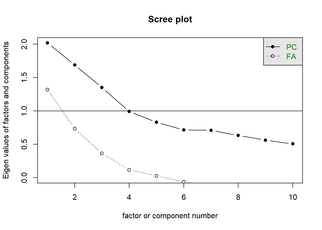
The horizontal line is an additional suggestion that we should keep all components for which the eigenvalue is >1. This is known as “Kaiser’s Criterion”
Parallel analysis
Rabbit Hole: What is parallel analysis?
Parallel analysis involves simulating lots of datasets of the same dimension but in which the variables are uncorrelated. For each of these simulations, a PCA is conducted on its correlation matrix, and the eigenvalues are extracted. We can then compare our eigenvalues from the PCA on our actual data to the average eigenvalues across these simulations. In theory, for uncorrelated variables, no components should explain more variance than any others, and eigenvalues should be equal to 1. In reality, variables are rarely truly uncorrelated, and so there will be slight variation in the magnitude of eigenvalues simply due to chance. The parallel analysis method suggests keeping those components for which the eigenvalues are greater than those from the simulations.
Parallel analysis can be conducted in R using the fa.parallel() function.
As with the scree plots, it presents this information for both orthogonal components (PCA) and correlated factors (EFA):
fa.parallel(distress_data)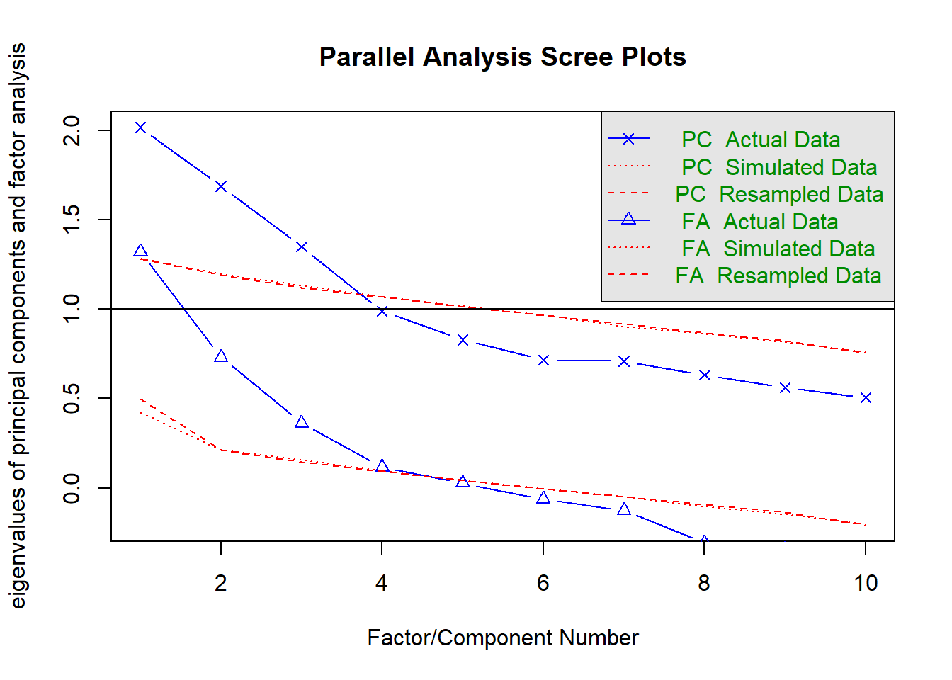
Parallel analysis suggests that the number of factors = 3 and the number of components = 3 NOTE: Parallel analysis will sometimes tend to over-extract (suggest too many components)
MAP
Rabbit Hole: What is MAP?
The Minimum Average Partial (MAP) test computes the partial correlation matrix (adjusting for and removing a component from the correlation matrix), sequentially partialling out each component. At each step, the partial correlations are squared and their average is computed.
At first, the components which are removed will be those that are most representative of the shared variance between 2+ variables, meaning that the “average squared partial correlation” will decrease. At some point in the process, the components being removed will begin represent variance that is specific to individual variables, meaning that the average squared partial correlation will increase.
The MAP method is to keep the number of components for which the average squared partial correlation is at the minimum.
We can conduct MAP in R using the VSS() function.
For PCA:
VSS(distress_data,
    rotate = "none", fm = "pc",
    plot = FALSE)
For EFA:
VSS(distress_data,
    rotate = "oblimin", fm = "ml",
    plot = FALSE)
There is a lot of other information in the output from VSS() too. We just want to focus on the map column, and the printed statement that tells us that the “Velicer MAP achieves a minimum” at a specific number of factors.
...
...
The Velicer MAP achieves a minimum of ???  with ???? factors
...
Statistics by number of factors
  vss1 vss2   map dof    ...    ...
1 ...  ...  0.030  ..    ...     ...
2 ...  ...  0.038  ..    ...     ...
3 ...  ...  0.052  ..    ...     ...
4 ...  ...  0.087  ..    ...     ...
5 ...  ...  0.119  ..    ...     ...
6 ...  ...  0.179  ..    ...     ...
. ...  ...    ...  ..    ...     ...
. ...  ...    ...  ..    ...     ...
NOTE: The MAP method will sometimes tend to under-extract (suggest too few components)
Summary
TODO table