Analysis Example 3: Many trials

Each of these pages provides an analysis run through for a different type of design. Each document is structured in the same way:

First the data and research context is introduced. For the purpose of these tutorials, we will only use examples where the data can be shared - either because it is from an open access publication, or because it is unpublished or simulated.
Second, we go through any tidying of the data that is required, before creating some brief descriptives and visualizations of the raw data.
Then, we conduct an analysis. Where possible, we translate the research questions into formal equations prior to fitting the models in lme4. Model comparisons are conducted, along with checks of distributional assumptions on our model residuals.
Finally, we visualize and interpret our analysis.

Please note that there will be only minimal explanation of the steps undertaken here, as these pages are intended as example analyses rather than additional labs readings. Please also be aware that there are many decisions to be made throughout conducting analyses, and it may be the case that you disagree with some of the choices we make here. As always with these things, it is how we justify our choices that is important. We warmly welcome any feedback and suggestions to improve these examples: please email ug.ppls.stats@ed.ac.uk.

Overview

This data comes from an undergraduate dissertation student. She ran an experiment looking at the way people’s perception of the size of models influences the price they are willing to pay for products. Participants saw a series of pictures of a number of items of clothing. The images had been manipulated so that (a) all pictures were of the same model, and (b) the size of the model differed from a 6 to 16. In total participants saw 54 images. During the study, each picture was presented to participants with a sliding scale from 0 to 100 underneath. Participants simply had to drag the cursor to the appropriate point on the slide to indicate how much they would pay for the garment.

This data was collected using Qualtrics. The resultant output was a wide format data set where each participant (n=120) is a row and each item (n=54) is a column. Along with each of these questions were a series of demographic variables, and two short survey measures assessing participants attitude to thinness.

The main ideas we were interested in looking at were whether:

participants would pay more for garments on thinner models
participants would pay more for items when the model size matched their actual size
participants would pay more for items when the model size matched their ideal size
the extent to which participants idealize thin figures would moderate (ii)

Data Wrangling

Unlike some of our examples, there was some fairly serious data cleaning needed with this data set. So let’s work through it.

The data is available at https://uoepsy.github.io/data/data_HA.csv

Code

library(tidyverse)
df <- read_csv("https://uoepsy.github.io/data/data_HA.csv")
head(df)

# A tibble: 6 × 116
  Respons…¹ Gender   Age Dress…² Top_1…³ Botto…⁴ Dress…⁵ Botto…⁶ Top_6…⁷ Dress…⁸
  <chr>      <dbl> <dbl>   <dbl>   <dbl>   <dbl>   <dbl>   <dbl>   <dbl>   <dbl>
1 P_ID1001       1    22      45      24      30      30      20      17      15
2 P_ID1002       1    20      30      19       9      52       0       5      16
3 P_ID1003       1    21      30      12       4      18      20       8      12
4 P_ID1004       1    21      39      30      30      45      25      20      25
5 P_ID1005       1    23      10       5      15       7      15       5      20
6 P_ID1006       1    43      40      30      45      60      35      25      30
# … with 106 more variables: Dress_12...11 <dbl>, Bottom_12...12 <dbl>,
#   Top_10...13 <dbl>, Top_8...14 <dbl>, Bottom_6...15 <dbl>,
#   Bottom_8...16 <dbl>, Dress_14...17 <dbl>, Top_16...18 <dbl>,
#   Bottom_6...19 <dbl>, Bottom_14...20 <dbl>, Top_8...21 <dbl>,
#   Dress_8...22 <dbl>, Top_12...23 <dbl>, Top_14...24 <dbl>,
#   Dress_16...25 <dbl>, Top_10...26 <dbl>, Top_14...27 <dbl>,
#   Dress_8...28 <dbl>, Dress_16...29 <dbl>, Bottom_12...30 <dbl>, …

First things first, let’s use a handy package to change all our variable names to a nice easy “snake_case”:

Code

library(janitor)
df <- clean_names(df)
head(df)

# A tibble: 6 × 116
  respons…¹ gender   age dress…² top_1…³ botto…⁴ dress…⁵ botto…⁶ top_6_9 dress…⁷
  <chr>      <dbl> <dbl>   <dbl>   <dbl>   <dbl>   <dbl>   <dbl>   <dbl>   <dbl>
1 P_ID1001       1    22      45      24      30      30      20      17      15
2 P_ID1002       1    20      30      19       9      52       0       5      16
3 P_ID1003       1    21      30      12       4      18      20       8      12
4 P_ID1004       1    21      39      30      30      45      25      20      25
5 P_ID1005       1    23      10       5      15       7      15       5      20
6 P_ID1006       1    43      40      30      45      60      35      25      30
# … with 106 more variables: dress_12_11 <dbl>, bottom_12_12 <dbl>,
#   top_10_13 <dbl>, top_8_14 <dbl>, bottom_6_15 <dbl>, bottom_8_16 <dbl>,
#   dress_14_17 <dbl>, top_16_18 <dbl>, bottom_6_19 <dbl>, bottom_14_20 <dbl>,
#   top_8_21 <dbl>, dress_8_22 <dbl>, top_12_23 <dbl>, top_14_24 <dbl>,
#   dress_16_25 <dbl>, top_10_26 <dbl>, top_14_27 <dbl>, dress_8_28 <dbl>,
#   dress_16_29 <dbl>, bottom_12_30 <dbl>, dress_6_31 <dbl>,
#   bottom_14_32 <dbl>, bottom_8_33 <dbl>, top_16_34 <dbl>, …

Our next job is to cut out a few variables that we will not work with in this example. These are a set of questions asking about clothing preferences. They all end in p and appear at the end of the data set.

Code

df1 <- 
  df %>%
  select(-ends_with("p"))

Now we want to create scores for the two surveys scored using Likert-type scales. We’re going to take the means of these scales as our scores:

Code

# TI score
df1 <- 
  df1 %>%
  select(contains("_tii")) %>%
  rowMeans(., na.rm=T) %>%
  bind_cols(df1, tii_score = .)
         
# MA score
df1 <- 
  df1 %>%
  select(contains("_mo")) %>%
  rowMeans(., na.rm=T) %>%
  bind_cols(df1, ma_score = .)

Next, we need to make some changes to the coding of current and ideal size

Code

df1 <- 
  df1 %>%
  mutate(
    c.size = recode(current_size, 6, 8, 10, 12, 14, 16),
    i.size = recode(ideal_size,  6, 8, 10, 12, 14, 16)
  )

Always sensible to check our changes:

Code

df1 %>%
  select(current_size, ideal_size, c.size, i.size)

# A tibble: 120 × 4
   current_size ideal_size c.size i.size
          <dbl>      <dbl>  <dbl>  <dbl>
 1            3          2     10      8
 2            1          1      6      6
 3            2          1      8      6
 4            2          1      8      6
 5            3          2     10      8
 6            4          3     12     10
 7            3          2     10      8
 8            2          2      8      8
 9            5          3     14     10
10            3          2     10      8
# … with 110 more rows

Excellent, that has worked.

Our next step (and this one is not strictly necessary) is that we are going to aggregate over the different types of top, bottoms and dresses. We could treat each individual garment of clothing as exactly that, but in this instance it was decided that this was not of interest, and to simplify the models, we would create scores for each broad category by size.

Code

df1 <- 
  df1 %>%
  mutate(top_S6 = rowMeans(.[names(df1)[grepl("top_6",names(df1))]]),
         top_S8 = rowMeans(.[names(df1)[grepl("top_8",names(df1))]]),
         top_S10 = rowMeans(.[names(df1)[grepl("top_10",names(df1))]]),
         top_S12 = rowMeans(.[names(df1)[grepl("top_12",names(df1))]]),
         top_S14 = rowMeans(.[names(df1)[grepl("top_14",names(df1))]]),
         top_S16 = rowMeans(.[names(df1)[grepl("top_16",names(df1))]]),
         bottom_S6 = rowMeans(.[names(df1)[grepl("bottom_6",names(df1))]]),
         bottom_S8 = rowMeans(.[names(df1)[grepl("bottom_8",names(df1))]]),
         bottom_S10 = rowMeans(.[names(df1)[grepl("bottom_10",names(df1))]]),
         bottom_S12 = rowMeans(.[names(df1)[grepl("bottom_12",names(df1))]]),
         bottom_S14 = rowMeans(.[names(df1)[grepl("bottom_14",names(df1))]]),
         bottom_S16 = rowMeans(.[names(df1)[grepl("bottom_16",names(df1))]]),
         dress_S6 = rowMeans(.[names(df1)[grepl("dress_6",names(df1))]]),
         dress_S8 = rowMeans(.[names(df1)[grepl("dress_8",names(df1))]]),
         dress_S10 = rowMeans(.[names(df1)[grepl("dress_10",names(df1))]]),
         dress_S12 = rowMeans(.[names(df1)[grepl("dress_12",names(df1))]]),
         dress_S14 = rowMeans(.[names(df1)[grepl("dress_14",names(df1))]]),
         dress_S16 = rowMeans(.[names(df1)[grepl("dress_16",names(df1))]]),
         )

At this point, our next big step is to make the data long. But I am also going to make this a little more manageable by trimming out the variables we do not need. We want ID and age, gender is constant (all female sample), so we do not need this, and then we want the variables we have just created.

Code

df2 <- 
  df1 %>%
  select(response_id, age, 99:120)

df2

# A tibble: 120 × 24
   response_id   age tii_s…¹ ma_sc…² c.size i.size top_S6 top_S8 top_S10 top_S12
   <chr>       <dbl>   <dbl>   <dbl>  <dbl>  <dbl>  <dbl>  <dbl>   <dbl>   <dbl>
 1 P_ID1001       22    2.63    1.78     10      8  20.7    16.3    21.7   20   
 2 P_ID1002       20    3       2.44      6      6   7.67   12.3    10     17.3 
 3 P_ID1003       21    2.6     1.78      8      6  16.7    10.3     9     11.7 
 4 P_ID1004       21    2.27    1.78      8      6  23.3    20      18.3   23.3 
 5 P_ID1005       23    2.87    2.56     10      8   6.33   10.7    11      8.33
 6 P_ID1006       43    2.73    2.22     12     10  28.3    25      41.7   30   
 7 P_ID1007       55    2.93    1.89     10      8  23.3    28.3    23.3   23.3 
 8 P_ID1008       20    3.03    2.11      8      8  21.3    20.7    19     23   
 9 P_ID1009       48    2.7     2.89     14     10  45.7    20.3    26.7   57   
10 P_ID1010       21    2.37    2        10      8  15.3    16.7    18.3   13.3 
# … with 110 more rows, 14 more variables: top_S14 <dbl>, top_S16 <dbl>,
#   bottom_S6 <dbl>, bottom_S8 <dbl>, bottom_S10 <dbl>, bottom_S12 <dbl>,
#   bottom_S14 <dbl>, bottom_S16 <dbl>, dress_S6 <dbl>, dress_S8 <dbl>,
#   dress_S10 <dbl>, dress_S12 <dbl>, dress_S14 <dbl>, dress_S16 <dbl>, and
#   abbreviated variable names ¹tii_score, ²ma_score

OK, now we need to get the data from wide to long format.

Code

df_long <- 
  df2 %>%
  pivot_longer(top_S6:dress_S16, names_to = "garment",values_to = "price")

df_long

# A tibble: 2,160 × 8
   response_id   age tii_score ma_score c.size i.size garment    price
   <chr>       <dbl>     <dbl>    <dbl>  <dbl>  <dbl> <chr>      <dbl>
 1 P_ID1001       22      2.63     1.78     10      8 top_S6      20.7
 2 P_ID1001       22      2.63     1.78     10      8 top_S8      16.3
 3 P_ID1001       22      2.63     1.78     10      8 top_S10     21.7
 4 P_ID1001       22      2.63     1.78     10      8 top_S12     20  
 5 P_ID1001       22      2.63     1.78     10      8 top_S14     15.3
 6 P_ID1001       22      2.63     1.78     10      8 top_S16     17  
 7 P_ID1001       22      2.63     1.78     10      8 bottom_S6   21.7
 8 P_ID1001       22      2.63     1.78     10      8 bottom_S8   18  
 9 P_ID1001       22      2.63     1.78     10      8 bottom_S10  30  
10 P_ID1001       22      2.63     1.78     10      8 bottom_S12  20  
# … with 2,150 more rows

This looks good, but we now need to have variables that code for size and item type.

Code

df_analysis <- 
  df_long %>%
  separate(garment, c("item", "size"), "_S")

And check….

Code

df_analysis

# A tibble: 2,160 × 9
   response_id   age tii_score ma_score c.size i.size item   size  price
   <chr>       <dbl>     <dbl>    <dbl>  <dbl>  <dbl> <chr>  <chr> <dbl>
 1 P_ID1001       22      2.63     1.78     10      8 top    6      20.7
 2 P_ID1001       22      2.63     1.78     10      8 top    8      16.3
 3 P_ID1001       22      2.63     1.78     10      8 top    10     21.7
 4 P_ID1001       22      2.63     1.78     10      8 top    12     20  
 5 P_ID1001       22      2.63     1.78     10      8 top    14     15.3
 6 P_ID1001       22      2.63     1.78     10      8 top    16     17  
 7 P_ID1001       22      2.63     1.78     10      8 bottom 6      21.7
 8 P_ID1001       22      2.63     1.78     10      8 bottom 8      18  
 9 P_ID1001       22      2.63     1.78     10      8 bottom 10     30  
10 P_ID1001       22      2.63     1.78     10      8 bottom 12     20  
# … with 2,150 more rows

Finally, our last couple of steps. First, we want to calculate a couple of binary variables that code whether a give item being rated matches a participants actual or ideal size; second, we need to make our item variable a factor, and third, let’s standardize our scale scores for idealization of thinness.

Code

df_analysis <- 
  df_analysis %>%
  mutate(
    c.match = factor(if_else(c.size == size, 1, 0)),
    i.match = factor(if_else(i.size == size, 1, 0)),
    sizefactor = factor(size, levels=c("6","8","10","12","14","16")),
    size = scale(as.numeric(as.character(size))),
    item = as.factor(item),
    id = response_id,
    tii_scorez = scale(tii_score),
    ma_scorez = scale(ma_score)
  )

df_analysis[,c(1,5:11)]

# A tibble: 2,160 × 8
   response_id c.size i.size item   size[,1] price c.match i.match
   <chr>        <dbl>  <dbl> <fct>     <dbl> <dbl> <fct>   <fct>  
 1 P_ID1001        10      8 top      -1.46   20.7 0       0      
 2 P_ID1001        10      8 top      -0.878  16.3 0       1      
 3 P_ID1001        10      8 top      -0.293  21.7 1       0      
 4 P_ID1001        10      8 top       0.293  20   0       0      
 5 P_ID1001        10      8 top       0.878  15.3 0       0      
 6 P_ID1001        10      8 top       1.46   17   0       0      
 7 P_ID1001        10      8 bottom   -1.46   21.7 0       0      
 8 P_ID1001        10      8 bottom   -0.878  18   0       1      
 9 P_ID1001        10      8 bottom   -0.293  30   1       0      
10 P_ID1001        10      8 bottom    0.293  20   0       0      
# … with 2,150 more rows

There’s a debate to be had about whether we should consider our size variable to be numeric or a factor. It could be argued that the sizes of clothing are distinct categories, and that the scale might not be regular (e.g. size 10 is not the same amount bigger than size 8 as size 8 is from size 6). On the other hand, clothing sizes can also be considered points on an underlying latent continuous variable, which might lead you to want to treat it as numeric. Personally, I would want to know exactly how the participants were presented with the sizes - if they were shown the images and the size of the garment was made explicit for each item, then I would be inclined to consider them distinct categories. However, if participants were not explicitly aware of the size of each item, and it was only the size of the model they saw that varied in their size, I am tempted to treat it numerically.

Descriptives

Let’s look at the average price paid by item type and size:

Code

df_analysis %>%
  group_by(size, item) %>%
  summarize(
    price = mean(price, na.rm=T)
  ) %>%
  arrange(item)

# A tibble: 18 × 3
# Groups:   size [6]
   size[,1] item   price
      <dbl> <fct>  <dbl>
 1   -1.46  bottom  26.1
 2   -0.878 bottom  25.7
 3   -0.293 bottom  23.7
 4    0.293 bottom  24.0
 5    0.878 bottom  24.1
 6    1.46  bottom  22.5
 7   -1.46  dress   28.2
 8   -0.878 dress   27.3
 9   -0.293 dress   26.2
10    0.293 dress   27.3
11    0.878 dress   25.8
12    1.46  dress   26.5
13   -1.46  top     18.6
14   -0.878 top     18.1
15   -0.293 top     20.0
16    0.293 top     19.1
17    0.878 top     19.2
18    1.46  top     19.3

This looks a lot like we are seeing difference, averaged across all participants, in the price they would pay for different types of garment, but not a lot of difference by size.

We can also calculate the ICC’s

Code

library(lme4)
m0 <- lmer(price ~ 1 + 
             (1|id) + (1|item),
           data = df_analysis)
ICC <- as.data.frame(VarCorr(m0))

For participant:

Code

round((ICC[1,4]/sum(ICC[,4]))*100, 2)

[1] 53.99

And item:

Code

round((ICC[2,4]/sum(ICC[,4]))*100, 2)

[1] 14.36

So we can see we have a lot of between person variation, and some between item variation in our data. This suggests that there is potential value in our level 2 predictors concerning both the items and between person characteristics.

Visualizations

There are too many ways to visualize this data! Here are just a few:

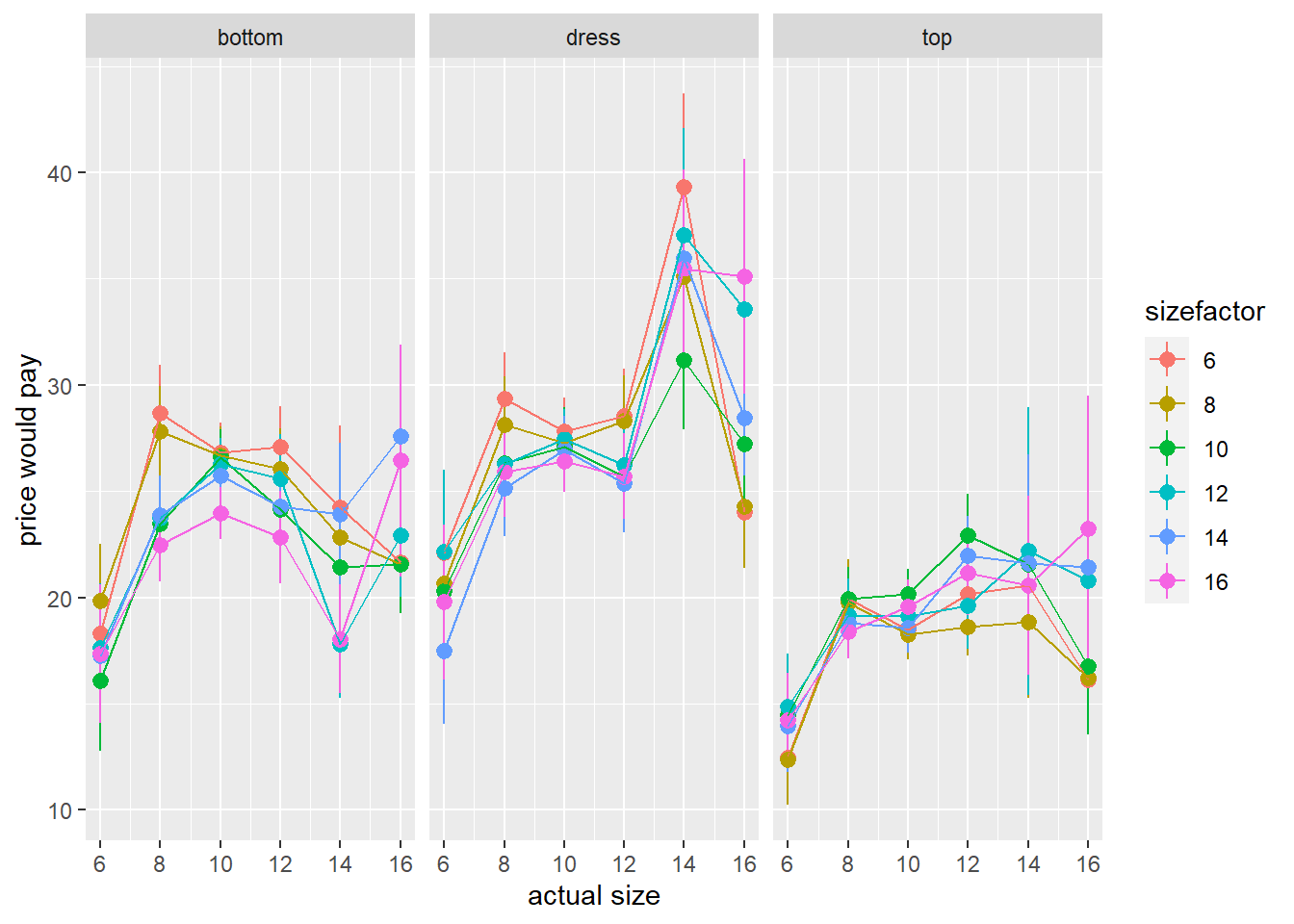
Code

ggplot(df_analysis, aes(x=c.size, y=price,col=sizefactor))+
  stat_summary(geom="pointrange")+
  stat_summary(geom="path")+
  facet_grid(~item)+
  labs(x="actual size",y="price would pay")

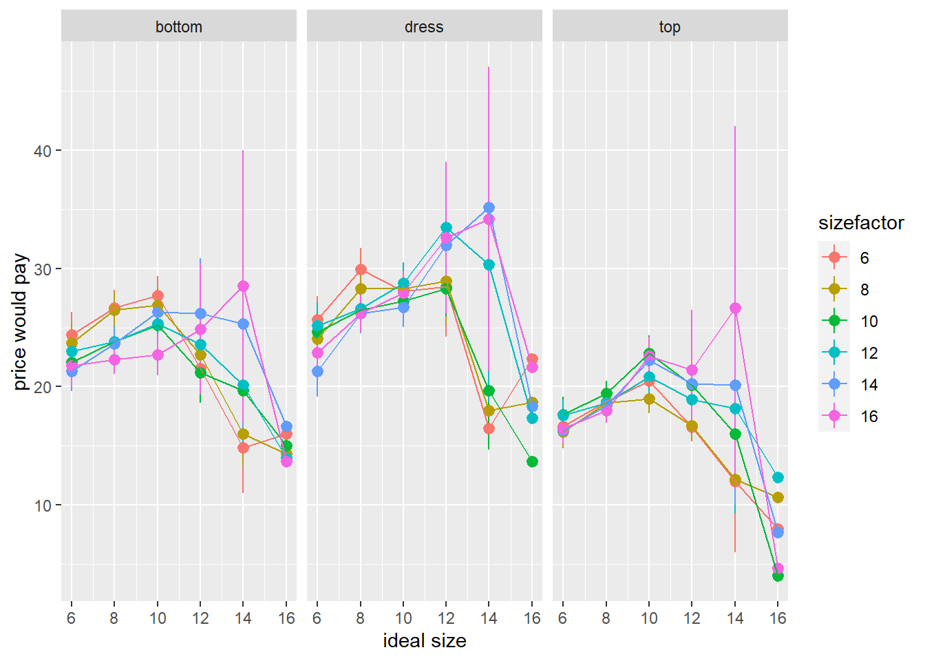
Code

ggplot(df_analysis, aes(x=i.size, y=price,col=sizefactor))+
  stat_summary(geom="pointrange")+
  stat_summary(geom="path")+
  facet_grid(~item)+
  labs(x="ideal size",y="price would pay")

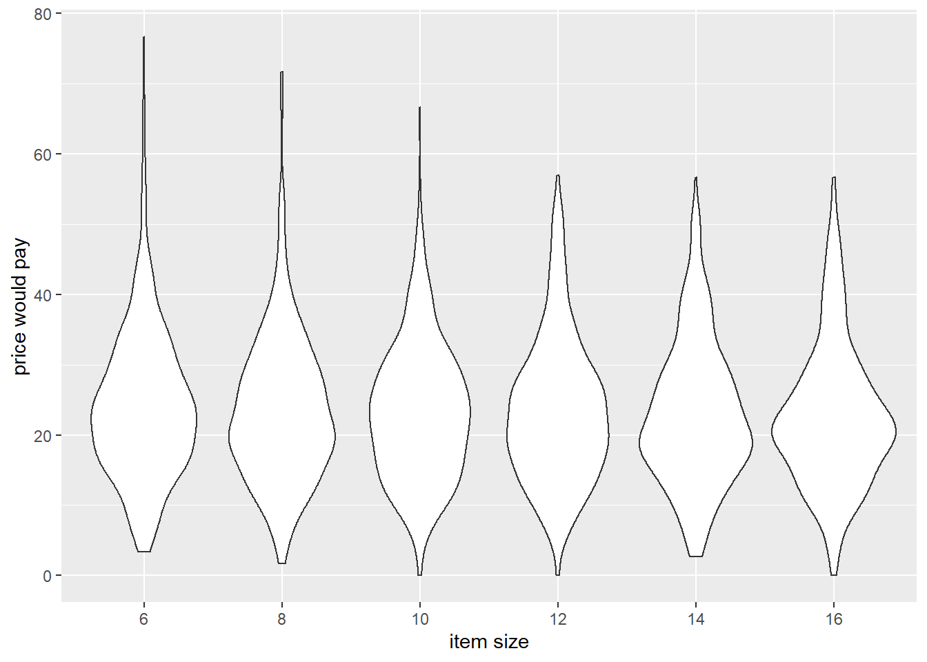
Remember, however, that we had some research questions to consider!

participants would pay more for garments on thinner models

Code

ggplot(df_analysis, aes(x=sizefactor, y=price))+
  geom_violin()+
  labs(x="item size",y="price would pay")

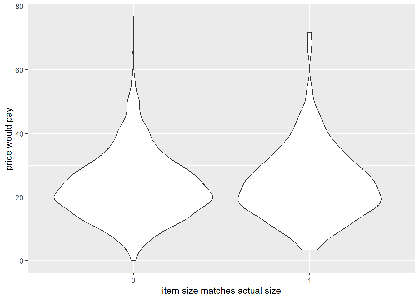
participants would pay more for items when the model size matched their actual size

Code

ggplot(df_analysis, aes(x=factor(c.match), y=price))+
  geom_violin()+
  labs(x="item size matches actual size",y="price would pay")

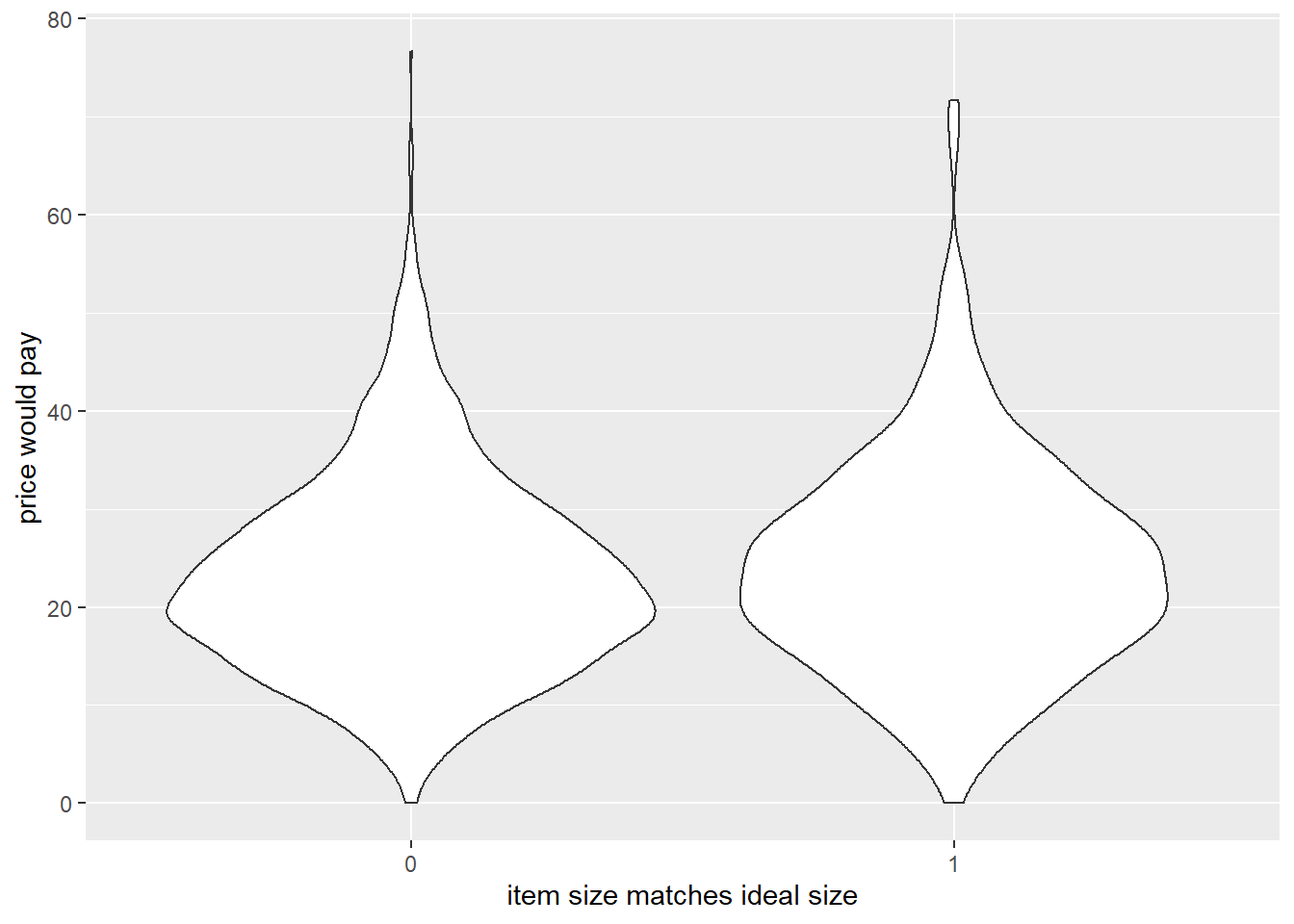
participants would pay more for items when the model size matched their ideal size

Code

ggplot(df_analysis, aes(x=factor(i.match), y=price))+
  geom_violin()+
  labs(x="item size matches ideal size",y="price would pay")

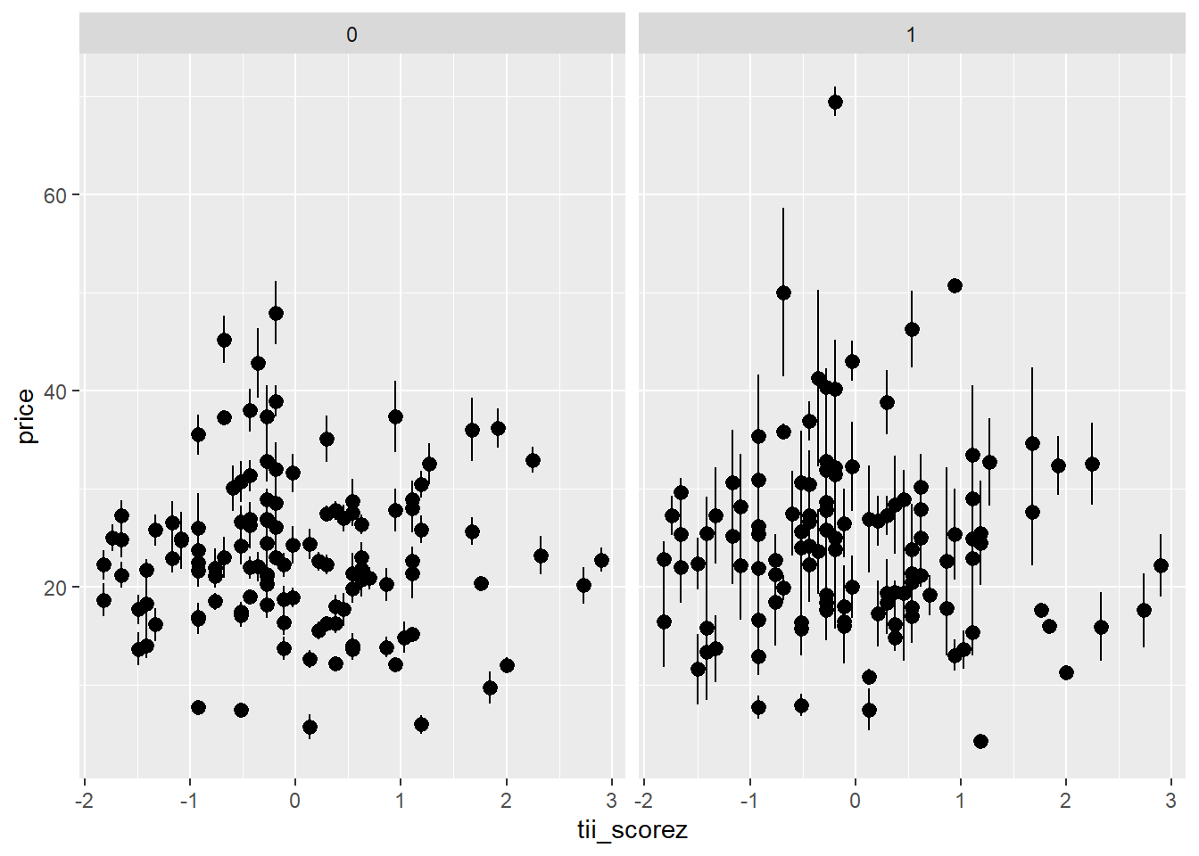
the extent to which participants idealize thin figures would moderate (ii)

Code

ggplot(df_analysis, aes(x=tii_scorez, y=price))+
  stat_summary(geom="pointrange",aes(group=id))+ # want a mean per participant, rather than each individual point
  facet_grid(~c.match)

Code

  labs(x="thinness idealization score",y="price would pay")

$x
[1] "thinness idealization score"

$y
[1] "price would pay"

attr(,"class")
[1] "labels"

Analysis

Equations

Why item as a fixed effect and not by-item random intercepts (e.g.(1 | item))? It is debatable how you decide to treat item here. It could be argued that the different item types (dress/top/bottom, etc) represent a sample from some broader population of garment types, and as such should be modeled as random effects (especially given that we are not interested in specific parameter estimates for differences between item types).

However, we only have 3 different types of item, and it is important to remember that having (1|item) will involve estimating variance components based on these. Variance estimates will be less stable with such a small number of groups. There’s no hard rule to follow here about “how many groups is enough” (some people suggest 5 or 6 at least), but personally I would be inclined to use item as a fixed effect.

We should also consider the possibility that certain items should be less desirable to purchase when in a smaller/bigger size. It may be that size differences are more salient, or more influential on our outcome variable, for certain types of item over others. This would involve adding the interaction between size and item type

$$ \[\begin{aligned} \operatorname{price}_{i[j]} =& \beta_{0i} + \beta_{1i}(\operatorname{item-size}_j) + \beta_{1}(\operatorname{item-type}_j) + \\ & \beta_{2}(\operatorname{item-size}_j \times \operatorname{item-type}_j) + \\ & \beta_{3i}(\operatorname{matches-actual-size}_j) + \\ & \beta_{4}(\operatorname{matches-ideal-size}_j) + \varepsilon_{i[j]}\\ \qquad \\ \beta_{0i} &= \gamma_{00} + \gamma_{01}(\operatorname{thin-idealisation-score}_i) + \zeta_{0i} \\ \beta_{1i} &= \gamma_{10} + \zeta_{1i}\\ \beta_{3i} &= \gamma_{30} + \gamma_{31}(\operatorname{thin-idealisation-score}_i)\\ & \text{for participant i = 1, } \dots \text{, I} \\ \end{aligned}\]

Fitting the models

We’re going to want to do lots of model comparisons, and for those we need all our models to be fitted on the same data. We’re going to use these variables:

Code

df_analysis <-
  df_analysis %>%
  filter(
    !is.na(size),
    !is.na(item),
    !is.na(c.match),
    !is.na(i.match),
    !is.na(tii_scorez),
    !is.na(id),
    !is.na(price)
  )

First, the effect of size. We’re going to treat size as a numeric variable here, in part because it makes our models less complex. It also allows us to model by-participant random effects of size (you can think of this as modeling participants as varying in the amount to which size influences the amount that they are prepared to pay).

Code

m0 <- lmer(price ~ 1 + item + 
             (1+size|id),
           data = df_analysis)
m1 <- lmer(price ~ 1 + item + size +
             (1 + size|id),
           data = df_analysis)
summary(m1)

Linear mixed model fit by REML ['lmerMod']
Formula: price ~ 1 + item + size + (1 + size | id)
   Data: df_analysis

REML criterion at convergence: 14045.7

Scaled residuals: 
    Min      1Q  Median      3Q     Max 
-4.5003 -0.5885 -0.0396  0.5259  5.1435 

Random effects:
 Groups   Name        Variance Std.Dev. Corr 
 id       (Intercept) 62.130   7.882         
          size         2.371   1.540    -0.07
 Residual             33.570   5.794         
Number of obs: 2130, groups:  id, 120

Fixed effects:
            Estimate Std. Error t value
(Intercept)  24.3845     0.7517  32.439
itemdress     2.6468     0.3081   8.590
itemtop      -5.3352     0.3073 -17.360
size         -0.4893     0.1887  -2.593

Correlation of Fixed Effects:
          (Intr) itmdrs itemtp
itemdress -0.204              
itemtop   -0.205  0.500       
size      -0.051  0.000  0.001

Code

anova(m0, m1)

Data: df_analysis
Models:
m0: price ~ 1 + item + (1 + size | id)
m1: price ~ 1 + item + size + (1 + size | id)
   npar   AIC   BIC  logLik deviance  Chisq Df Pr(>Chisq)  
m0    7 14065 14104 -7025.3    14051                       
m1    8 14060 14105 -7022.0    14044 6.6082  1    0.01015 *
---
Signif. codes:  0 '***' 0.001 '**' 0.01 '*' 0.05 '.' 0.1 ' ' 1

The interaction between size and item:

Code

m2 <- lmer(price ~ 1 +  item * size +
             (1+size|id),
           data = df_analysis)
summary(m2)

Linear mixed model fit by REML ['lmerMod']
Formula: price ~ 1 + item * size + (1 + size | id)
   Data: df_analysis

REML criterion at convergence: 14026.4

Scaled residuals: 
    Min      1Q  Median      3Q     Max 
-4.5043 -0.5804 -0.0377  0.5095  5.1433 

Random effects:
 Groups   Name        Variance Std.Dev. Corr 
 id       (Intercept) 62.135   7.883         
          size         2.392   1.547    -0.07
 Residual             33.240   5.765         
Number of obs: 2130, groups:  id, 120

Fixed effects:
               Estimate Std. Error t value
(Intercept)     24.3870     0.7514  32.454
itemdress        2.6449     0.3066   8.626
itemtop         -5.3370     0.3058 -17.451
size            -1.1062     0.2587  -4.277
itemdress:size   0.4740     0.3071   1.543
itemtop:size     1.3689     0.3058   4.477

Correlation of Fixed Effects:
            (Intr) itmdrs itemtp size   itmdr:
itemdress   -0.203                            
itemtop     -0.204  0.500                     
size        -0.038  0.002  0.002              
itemdrss:sz  0.001 -0.003 -0.002 -0.591       
itemtop:siz  0.001 -0.002 -0.002 -0.594  0.500

Code

anova(m1,m2)

Data: df_analysis
Models:
m1: price ~ 1 + item + size + (1 + size | id)
m2: price ~ 1 + item * size + (1 + size | id)
   npar   AIC   BIC  logLik deviance  Chisq Df Pr(>Chisq)    
m1    8 14060 14105 -7022.0    14044                         
m2   10 14043 14100 -7011.7    14023 20.613  2  3.341e-05 ***
---
Signif. codes:  0 '***' 0.001 '**' 0.01 '*' 0.05 '.' 0.1 ' ' 1

What about the effect of item size matching your current size:

Code

m3 <- lmer(price ~ 1 +  item * size + c.match +
             (1+size|id),
           data = df_analysis)
summary(m3)

Linear mixed model fit by REML ['lmerMod']
Formula: price ~ 1 + item * size + c.match + (1 + size | id)
   Data: df_analysis

REML criterion at convergence: 14023.1

Scaled residuals: 
    Min      1Q  Median      3Q     Max 
-4.4754 -0.5995 -0.0312  0.5075  5.1647 

Random effects:
 Groups   Name        Variance Std.Dev. Corr 
 id       (Intercept) 62.145   7.883         
          size         2.317   1.522    -0.08
 Residual             33.233   5.765         
Number of obs: 2130, groups:  id, 120

Fixed effects:
               Estimate Std. Error t value
(Intercept)     24.2782     0.7537  32.214
itemdress        2.6431     0.3066   8.621
itemtop         -5.3374     0.3058 -17.454
size            -1.0747     0.2580  -4.166
c.match1         0.6620     0.3494   1.895
itemdress:size   0.4736     0.3071   1.542
itemtop:size     1.3689     0.3058   4.477

Correlation of Fixed Effects:
            (Intr) itmdrs itemtp size   c.mtc1 itmdr:
itemdress   -0.202                                   
itemtop     -0.203  0.500                            
size        -0.048  0.002  0.002                     
c.match1    -0.076 -0.003 -0.001  0.064              
itemdrss:sz  0.001 -0.003 -0.002 -0.592  0.000       
itemtop:siz  0.001 -0.002 -0.002 -0.595  0.000  0.500

Compare models for current size match:

Code

anova(m2,m3)

Data: df_analysis
Models:
m2: price ~ 1 + item * size + (1 + size | id)
m3: price ~ 1 + item * size + c.match + (1 + size | id)
   npar   AIC   BIC  logLik deviance  Chisq Df Pr(>Chisq)  
m2   10 14043 14100 -7011.7    14023                       
m3   11 14042 14104 -7009.9    14020 3.5856  1    0.05828 .
---
Signif. codes:  0 '***' 0.001 '**' 0.01 '*' 0.05 '.' 0.1 ' ' 1

Or your ideal size:

Code

m4 <- lmer(price ~ 1 + item * size + c.match + i.match +
             (1+size|id),
           data = df_analysis)
summary(m4)

Linear mixed model fit by REML ['lmerMod']
Formula: price ~ 1 + item * size + c.match + i.match + (1 + size | id)
   Data: df_analysis

REML criterion at convergence: 14021.9

Scaled residuals: 
    Min      1Q  Median      3Q     Max 
-4.4705 -0.5911 -0.0355  0.5049  5.1828 

Random effects:
 Groups   Name        Variance Std.Dev. Corr 
 id       (Intercept) 62.171   7.885         
          size         2.281   1.510    -0.08
 Residual             33.244   5.766         
Number of obs: 2130, groups:  id, 120

Fixed effects:
               Estimate Std. Error t value
(Intercept)     24.2167     0.7556  32.050
itemdress        2.6439     0.3066   8.622
itemtop         -5.3369     0.3058 -17.450
size            -1.0264     0.2606  -3.938
c.match1         0.5972     0.3539   1.688
i.match1         0.4308     0.3650   1.180
itemdress:size   0.4736     0.3071   1.542
itemtop:size     1.3685     0.3058   4.475

Correlation of Fixed Effects:
            (Intr) itmdrs itemtp size   c.mtc1 i.mtc1 itmdr:
itemdress   -0.202                                          
itemtop     -0.203  0.500                                   
size        -0.058  0.002  0.002                            
c.match1    -0.064 -0.003 -0.001  0.038                     
i.match1    -0.069  0.002  0.001  0.156 -0.160              
itemdrss:sz  0.001 -0.003 -0.002 -0.586 -0.001  0.000       
itemtop:siz  0.001 -0.002 -0.002 -0.589  0.000 -0.001  0.500
optimizer (nloptwrap) convergence code: 0 (OK)
Model failed to converge with max|grad| = 0.00383895 (tol = 0.002, component 1)

Compare models for ideal size match:

Code

anova(m3,m4)

Data: df_analysis
Models:
m3: price ~ 1 + item * size + c.match + (1 + size | id)
m4: price ~ 1 + item * size + c.match + i.match + (1 + size | id)
   npar   AIC   BIC  logLik deviance Chisq Df Pr(>Chisq)
m3   11 14042 14104 -7009.9    14020                    
m4   12 14042 14110 -7009.2    14018 1.399  1     0.2369

Fixed effects for thin ideals:

Code

m5 <- lmer(price ~ 1 + item * size + c.match + i.match + tii_scorez + 
             (1+size|id),
           data = df_analysis)
summary(m5)

Linear mixed model fit by REML ['lmerMod']
Formula: price ~ 1 + item * size + c.match + i.match + tii_scorez + (1 +  
    size | id)
   Data: df_analysis

REML criterion at convergence: 14020.7

Scaled residuals: 
    Min      1Q  Median      3Q     Max 
-4.4719 -0.5907 -0.0357  0.5059  5.1829 

Random effects:
 Groups   Name        Variance Std.Dev. Corr 
 id       (Intercept) 62.695   7.918         
          size         2.279   1.510    -0.08
 Residual             33.245   5.766         
Number of obs: 2130, groups:  id, 120

Fixed effects:
               Estimate Std. Error t value
(Intercept)    24.21667    0.75848  31.928
itemdress       2.64389    0.30664   8.622
itemtop        -5.33684    0.30584 -17.450
size           -1.02641    0.26060  -3.939
c.match1        0.59704    0.35388   1.687
i.match1        0.43085    0.36497   1.181
tii_scorez     -0.07229    0.73246  -0.099
itemdress:size  0.47367    0.30714   1.542
itemtop:size    1.36846    0.30582   4.475

Correlation of Fixed Effects:
            (Intr) itmdrs itemtp size   c.mtc1 i.mtc1 t_scrz itmdr:
itemdress   -0.201                                                 
itemtop     -0.202  0.500                                          
size        -0.058  0.002  0.002                                   
c.match1    -0.064 -0.003 -0.001  0.038                            
i.match1    -0.068  0.002  0.001  0.156 -0.160                     
tii_scorez   0.000  0.000 -0.001  0.001  0.003 -0.001              
itemdrss:sz  0.001 -0.003 -0.002 -0.587 -0.001  0.000  0.000       
itemtop:siz  0.001 -0.002 -0.002 -0.589  0.000 -0.001  0.000  0.500

Compare models for thin ideal:

Code

anova(m4,m5)

Data: df_analysis
Models:
m4: price ~ 1 + item * size + c.match + i.match + (1 + size | id)
m5: price ~ 1 + item * size + c.match + i.match + tii_scorez + (1 + size | id)
   npar   AIC   BIC  logLik deviance  Chisq Df Pr(>Chisq)
m4   12 14042 14110 -7009.2    14018                     
m5   13 14044 14118 -7009.2    14018 0.0099  1     0.9208

Do they interact?

Code

m6 <- lmer(price ~ 1 + item * size + c.match + i.match + tii_scorez + c.match*tii_scorez + 
             (1+size|id),
           data = df_analysis)
summary(m6)

Linear mixed model fit by REML ['lmerMod']
Formula: price ~ 1 + item * size + c.match + i.match + tii_scorez + c.match *  
    tii_scorez + (1 + size | id)
   Data: df_analysis

REML criterion at convergence: 14019.8

Scaled residuals: 
    Min      1Q  Median      3Q     Max 
-4.4672 -0.5966 -0.0323  0.5021  5.1910 

Random effects:
 Groups   Name        Variance Std.Dev. Corr 
 id       (Intercept) 62.679   7.917         
          size         2.281   1.510    -0.08
 Residual             33.243   5.766         
Number of obs: 2130, groups:  id, 120

Fixed effects:
                    Estimate Std. Error t value
(Intercept)         24.20683    0.75845  31.916
itemdress            2.64336    0.30663   8.621
itemtop             -5.33608    0.30584 -17.448
size                -1.02537    0.26062  -3.934
c.match1             0.56650    0.35506   1.595
i.match1             0.51739    0.37448   1.382
tii_scorez          -0.01563    0.73458  -0.021
itemdress:size       0.47423    0.30713   1.544
itemtop:size         1.36867    0.30581   4.476
c.match1:tii_scorez -0.37423    0.36191  -1.034

Correlation of Fixed Effects:
            (Intr) itmdrs itemtp size   c.mtc1 i.mtc1 t_scrz itmdr: itmtp:
itemdress   -0.201                                                        
itemtop     -0.202  0.500                                                 
size        -0.056  0.002  0.002                                          
c.match1    -0.063 -0.003 -0.001  0.037                                   
i.match1    -0.070  0.002  0.002  0.153 -0.173                            
tii_scorez  -0.001  0.000  0.000  0.001 -0.003  0.016                     
itemdrss:sz  0.001 -0.003 -0.002 -0.586 -0.001  0.001  0.000              
itemtop:siz  0.001 -0.002 -0.002 -0.589  0.000 -0.001  0.000  0.500       
c.mtch1:t_s  0.013  0.002 -0.002 -0.004  0.082 -0.224 -0.076 -0.002 -0.001

And let’s just compare all at once, just for fun:

Code

anova(m0,m1,m2,m3,m4,m5,m6)

Data: df_analysis
Models:
m0: price ~ 1 + item + (1 + size | id)
m1: price ~ 1 + item + size + (1 + size | id)
m2: price ~ 1 + item * size + (1 + size | id)
m3: price ~ 1 + item * size + c.match + (1 + size | id)
m4: price ~ 1 + item * size + c.match + i.match + (1 + size | id)
m5: price ~ 1 + item * size + c.match + i.match + tii_scorez + (1 + size | id)
m6: price ~ 1 + item * size + c.match + i.match + tii_scorez + c.match * tii_scorez + (1 + size | id)
   npar   AIC   BIC  logLik deviance   Chisq Df Pr(>Chisq)    
m0    7 14065 14104 -7025.3    14051                          
m1    8 14060 14105 -7022.0    14044  6.6082  1    0.01015 *  
m2   10 14043 14100 -7011.7    14023 20.6131  2  3.341e-05 ***
m3   11 14042 14104 -7009.9    14020  3.5856  1    0.05828 .  
m4   12 14042 14110 -7009.2    14018  1.3990  1    0.23690    
m5   13 14044 14118 -7009.2    14018  0.0099  1    0.92076    
m6   14 14045 14125 -7008.7    14017  1.0720  1    0.30048    
---
Signif. codes:  0 '***' 0.001 '**' 0.01 '*' 0.05 '.' 0.1 ' ' 1

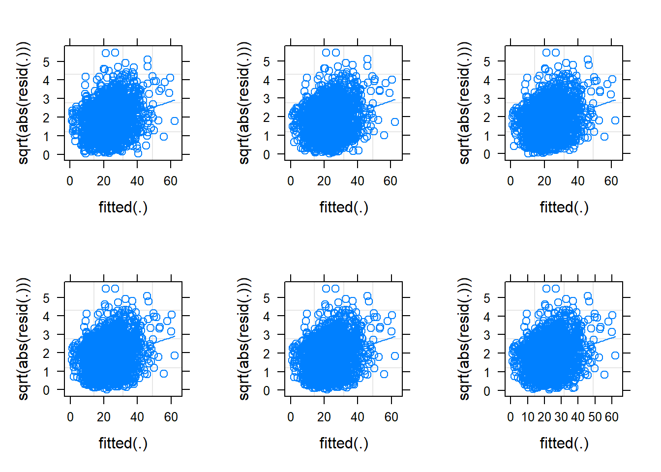
Check model(s)

Code

library(lattice)
library(gridExtra)
grid.arrange(
  plot(m1, sqrt(abs(resid(.)))~fitted(.), type = c("p","smooth")),
  plot(m2, sqrt(abs(resid(.)))~fitted(.), type = c("p","smooth")),
  plot(m3, sqrt(abs(resid(.)))~fitted(.), type = c("p","smooth")),
  plot(m4, sqrt(abs(resid(.)))~fitted(.), type = c("p","smooth")),
  plot(m5, sqrt(abs(resid(.)))~fitted(.), type = c("p","smooth")),
  plot(m6, sqrt(abs(resid(.)))~fitted(.), type = c("p","smooth")),
  ncol=3
)

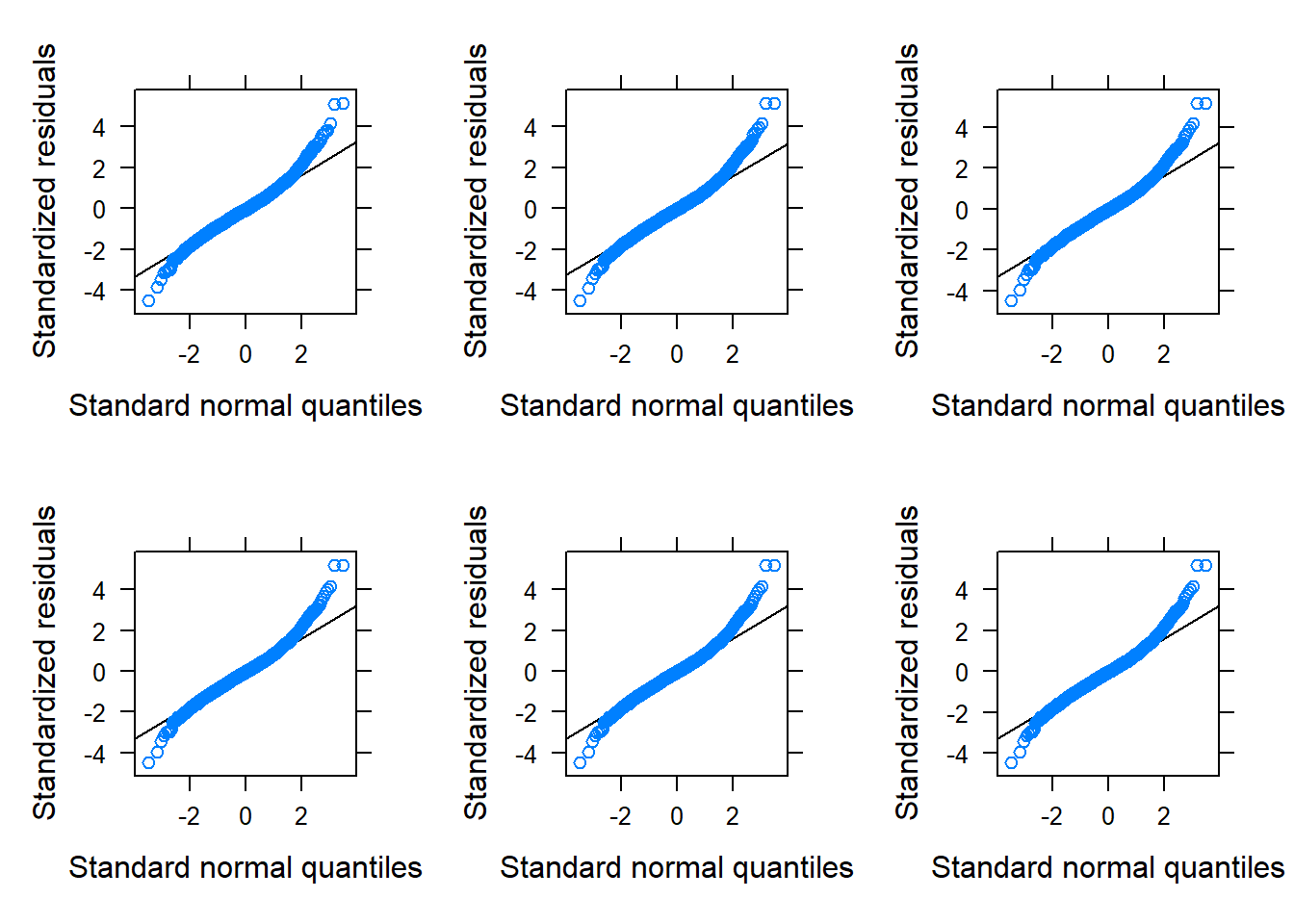
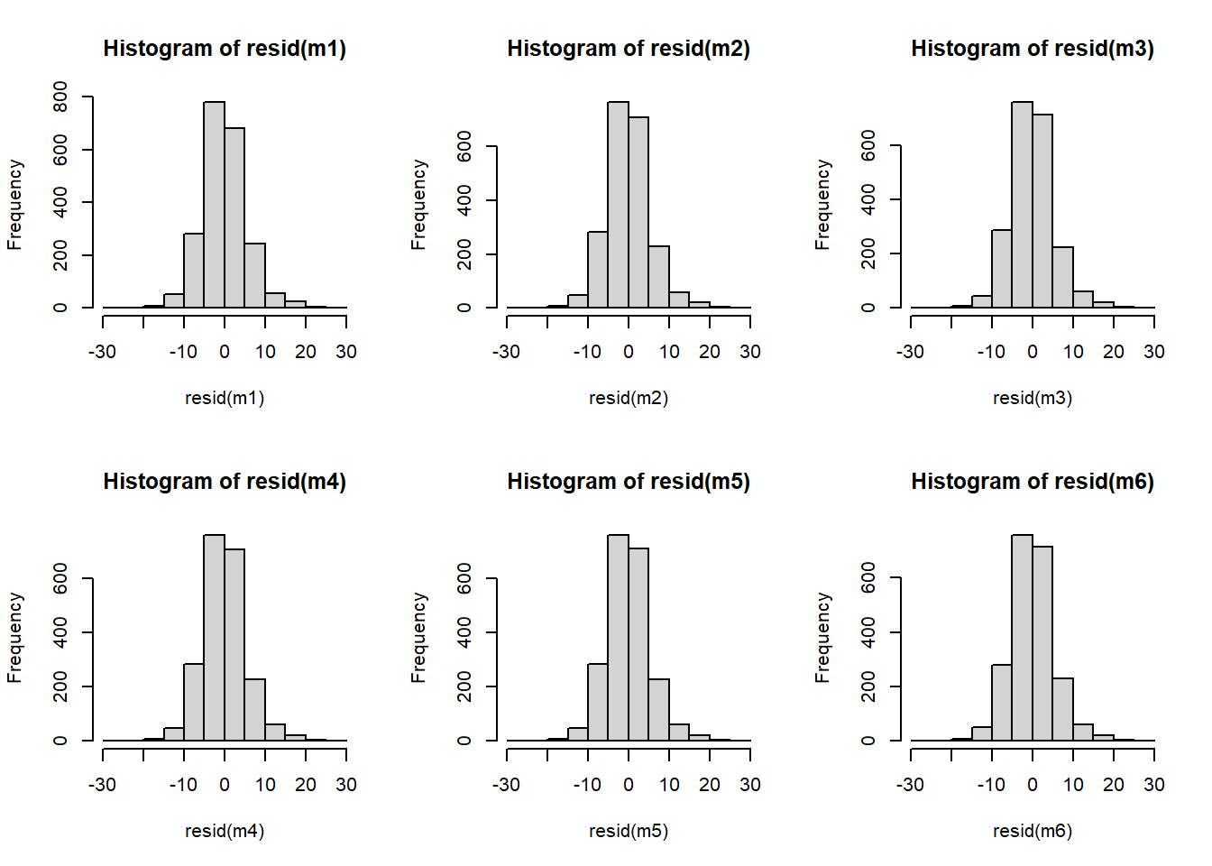
Code

grid.arrange(
  qqmath(m1),
  qqmath(m2),
  qqmath(m3),
  qqmath(m4),
  qqmath(m5),
  qqmath(m6),
  ncol=3
)

I might be a little concerned about our assumptions here. The QQplots look a little off in the tails, however, the histograms of residuals make it look okay:

For peace of mind, we could re-do the model comparisons with parametric bootstrapped model comparison for more reliable conclusions. This will assume that the model specified distribution of residuals ($\varepsilon \sim N(0, \sigma_\varepsilon)$) holds in the population

Code

library(pbkrtest)
PBmodcomp(m1, m0)

           stat df    p.value
LRT    6.605558  1 0.01016610
PBtest 6.605558 NA 0.01098901

Code

PBmodcomp(m2, m1)

           stat df      p.value
LRT    20.61468  2 3.338708e-05
PBtest 20.61468 NA 9.990010e-04

Code

PBmodcomp(m3, m2)

           stat df    p.value
LRT    3.585967  1 0.05826951
PBtest 3.585967 NA 0.07092907

Code

PBmodcomp(m4, m3)

           stat df   p.value
LRT    1.399085  1 0.2368768
PBtest 1.399085 NA 0.2317682

Code

PBmodcomp(m5, m4)

             stat df   p.value
LRT    0.00153228  1 0.9687753
PBtest 0.00153228 NA 0.9670330

Code

PBmodcomp(m6, m5)

           stat df   p.value
LRT    1.072739  1 0.3003275
PBtest 1.072739 NA 0.2857143

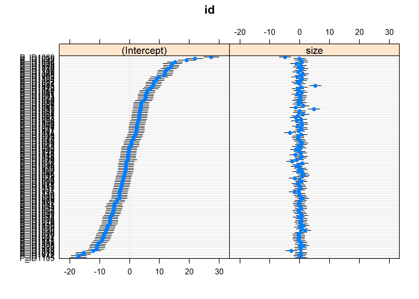
Visualise model(s)

Code

sjPlot::plot_model(m6)

Code

dotplot.ranef.mer(ranef(m6))

$id

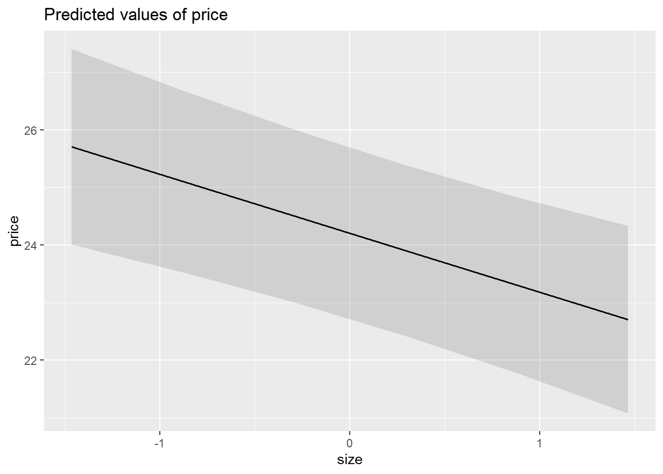
Code

library(sjPlot)
plot_model(m6, type = "pred")$size

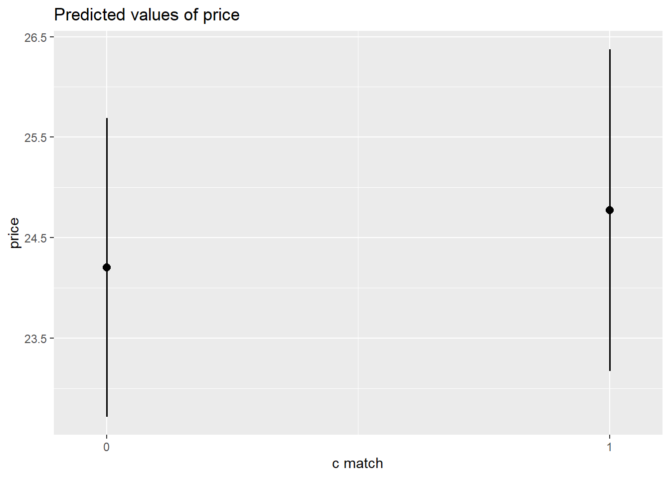
Code

plot_model(m6, type = "pred")$c.match

Code

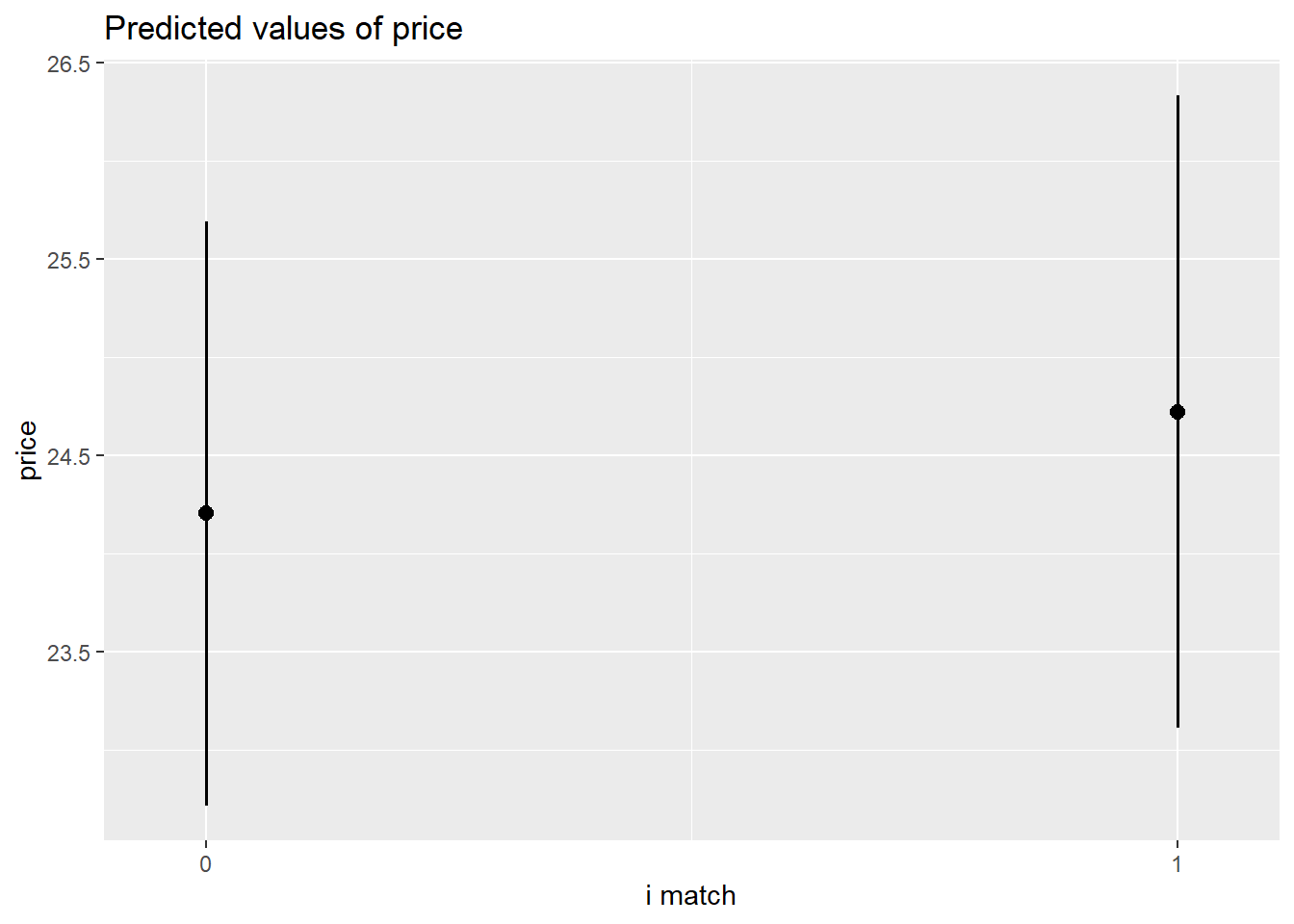
plot_model(m6, type = "pred")$i.match

Code

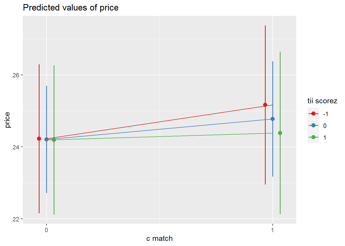
plot_model(m6, type = "pred", terms = c("c.match","tii_scorez [-1,0,1]")) +
   geom_path()

Interpret model(s)

The amount that participants indicated they would pay for a garment was modeled using multi-level linear regression models, with by-participant random intercepts and effects of garment size. After adjusting for effects on our outcome due to the garment-type (dress/top/bottom), inclusion of garment size as a fixed predictor was found to improve model fit (Parametric Bootstrap Likelihood Ratio = 6.61, p = 0.011). The effect of garment-size was found to differ between garment-types (inclusion of interaction term LRT 20.61, p <.001). After controlling for garment-type, -size and their interaction, neither the garments’ matching participants’ actual or ideal size, nor the extent to which participants idealized thin figures were found to predict the price they would pay, and the predicted interaction between actual-size matching and idealization of thin figures was not evidenced. Results of the full model are shown in Table 1.

Code

tab_model(m6, show.p = F, title="Table 1: Model results. Please note that 95% CIs are not bootstrapped")

Table 1: Model results. Please note that 95% CIs are not bootstrapped
	price
Predictors	Estimates	CI
(Intercept)	24.21	22.72 – 25.69
item [dress]	2.64	2.04 – 3.24
item [top]	-5.34	-5.94 – -4.74
size	-1.03	-1.54 – -0.51
c match [1]	0.57	-0.13 – 1.26
i match [1]	0.52	-0.22 – 1.25
tii scorez	-0.02	-1.46 – 1.42
item [dress] * size	0.47	-0.13 – 1.08
item [top] * size	1.37	0.77 – 1.97
c match [1] * tii scorez	-0.37	-1.08 – 0.34
Random Effects
σ²	33.24
τ₀₀ _id	62.68
τ₁₁ _id.size	2.28
ρ₀₁ _id	-0.08
ICC	0.66
N _id	120
Observations	2130
Marginal R² / Conditional R²	0.106 / 0.697