Recap of multilevel models

No specific exercises this week

This week, there aren’t any exercises, but there is a small recap reading of multilevel models, followed by some ‘flashcard’ type boxes to help you test your understanding of some of the key concepts.

Please use the lab sessions to go over exercises from previous weeks, as well as asking any questions about the content below.

Flashcards: lm to lmer

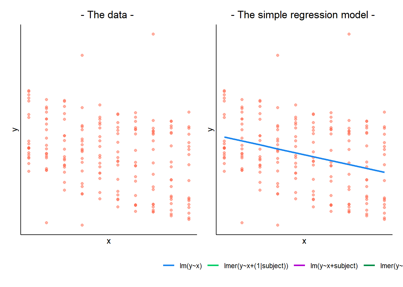
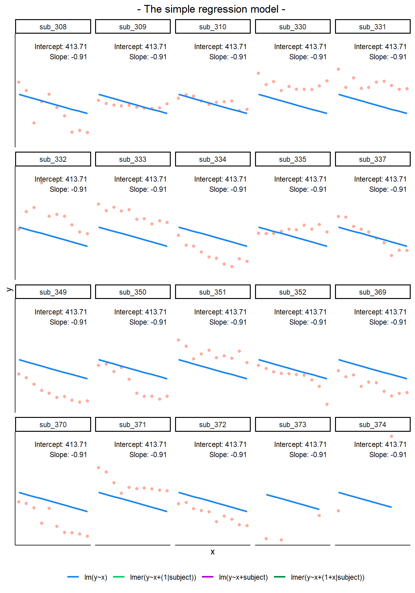
In a simple linear regression, there is only considered to be one source of random variability: any variability left unexplained by a set of predictors (which are modelled as fixed estimates) is captured in the model residuals.

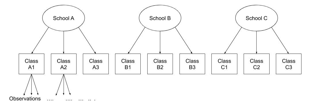
Multi-level (or ‘mixed-effects’) approaches involve modelling more than one source of random variability - as well as variance resulting from taking a random sample of observations, we can identify random variability across different groups of observations. For example, if we are studying a patient population in a hospital, we would expect there to be variability across the our sample of patients, but also across the doctors who treat them.

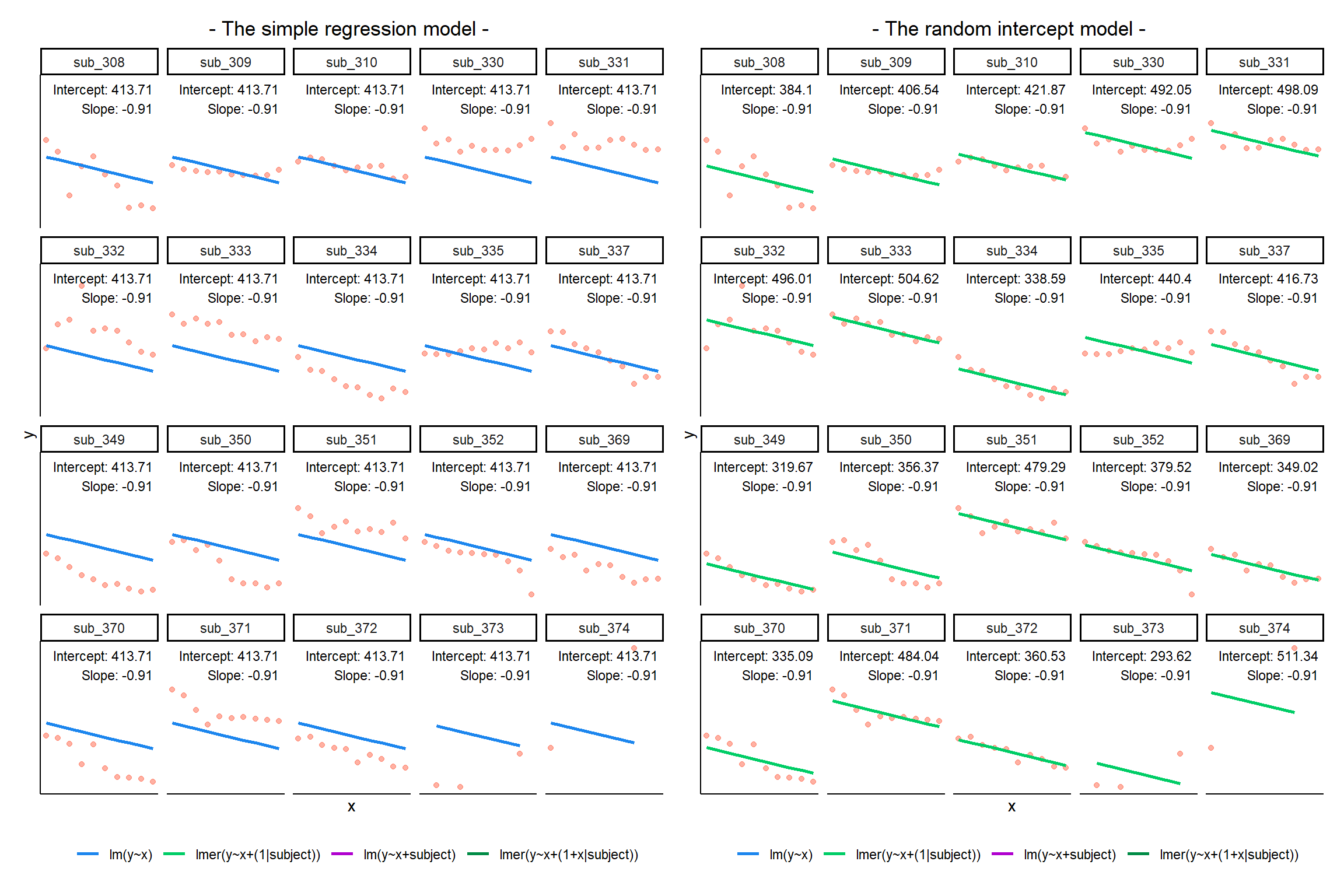
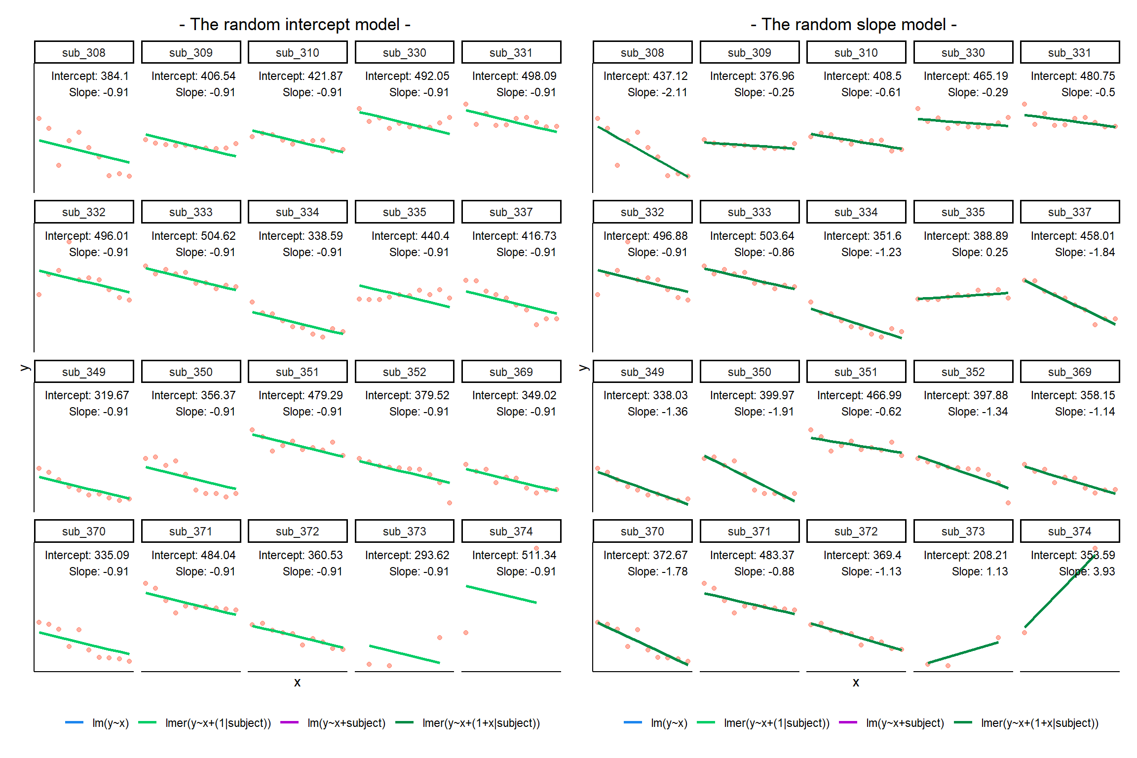
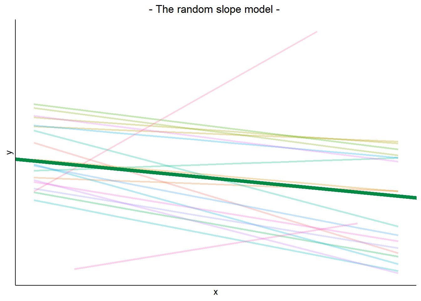
We can account for this variability by allowing the outcome to be lower/higher for each group (a random intercept) and by allowing the estimated effect of a predictor vary across groups (random slopes).

Before you expand each of the boxes below, think about how comfortable you feel with each concept.
This content is very cumulative, which means often going back to try to isolate the place which we need to focus efforts in learning.

Simple Linear Regression

Formula:

• $y_i={\beta }_0+{\beta }_1{x}_i+{ϵ}_i$

R command:

• lm(outcome ~ predictor, data = dataframe)

Note: this is the same as lm(outcome ~ 1 + predictor, data = dataframe). The 1 + is always there unless we specify otherwise (e.g., by using 0 +).

Clustered (multi-level) data

When our data is clustered (or ‘grouped’) such that datapoints are no longer independent, but belong to some grouping such as that of multiple observations from the same subject, we have multiple sources of random variability. A simple regression does not capture this.

If we separate out our data to show an individual plot for each grouping (in this data the grouping is by subjects), we can see how the fitted regression line from lm() is assumed to be the same for each group.

Random intercepts

By including a random-intercept term, we are letting our model estimate random variability around an average parameter (represented by the fixed effects) for the clusters.

Formula:
Level 1:

• $y_{ij}={\beta }_{0i}+{\beta }_{1i}{x}_{ij}+{ϵ}_{ij}$

Level 2:

• ${\beta }_{0i}={\gamma }_{00}+{\zeta }_{0i}$

Where the expected values of ${\zeta }_0$, and $ϵ$ are 0, and their variances are ${\sigma }_0^2$ and ${\sigma }_{ϵ}^2$ respectively. We will further assume that these are normally distributed.

We can now see that the intercept estimate ${\beta }_{0i}$ for a particular group $i$ is represented by the combination of a mean estimate for the parameter (${\gamma }_{00}$) and a random effect for that group (${\zeta }_{0i}$).

R command:

• lmer(outcome ~ predictor + (1 | grouping), data = dataframe)

Notice how the fitted line of the random intercept model has an adjustment for each subject.
Each subject’s line has been moved up or down accordingly.

Shrinkage

If you think about it, we might have done a similar thing to the random intercept with the tools we already had at our disposal, by using lm(y~x+subject). This would give us a coefficient for the difference between each subject and the reference level intercept, or we could extend this to lm(y~x*subject) to give us an adjustment to the slope for each subject.

However, the estimate of these models will be slightly different:

Why? One of the benefits of multi-level models is that our cluster-level estimates are shrunk towards the average depending on a) the level of across-cluster variation and b) the number of datapoints in clusters.

Random slopes

Formula:
Level 1:

• $y_{ij}={\beta }_{0i}+{\beta }_{1i}{x}_{ij}+{ϵ}_{ij}$

Level 2:

• ${\beta }_{0i}={\gamma }_{00}+{\zeta }_{0i}$
  
• ${\beta }_{1i}={\gamma }_{10}+{\zeta }_{1i}$

Where the expected values of ${\zeta }_0$, ${\zeta }_1$, and $ϵ$ are 0, and their variances are ${\sigma }_0^2$, ${\sigma }_1^2$, ${\sigma }_{ϵ}^2$ respectively. We will further assume that these are normally distributed.

As with the intercept ${\beta }_{0i}$, the slope of the predictor ${\beta }_{1i}$ is now modelled by a mean ${\gamma }_{10}$ and a random effect for each group (${\zeta }_{1i}$).

R command:

• lmer(outcome ~ predictor + (1 + predictor | grouping), data = dataframe)

Note: this is the same as lmer(outcome ~ predictor + (predictor | grouping), data = dataframe) . Like in the fixed-effects part, the 1 + is assumed in the random-effects part.

Fixed effects

The plot below show the fitted values for each subject from the random slopes model lmer(outcome ~ predictor + (1 + predictor | grouping), data = dataframe)

The thick green line shows the fixed intercept and slope around which the groups all vary randomly.

The fixed effects are the parameters that define the thick green line, and we can extract them using the fixef() function:

These are the overall intercept and slope.

fixef(random_slopes_model)

(Intercept)          x1 
405.7897675  -0.6722654 

Random effects

The plots below show the fitted values for each subject from each model that we have gone through in these expandable boxes (simple linear regression, random intercept, and random intercept & slope):

In the random-intercept model (center panel), the differences from each of the subjects’ intercepts to the fixed intercept (thick green line) have mean 0 and standard deviation ${\sigma }_0$. The standard deviation (and variance, which is ${\sigma }_0^2$) is what we see in the random effects part of our model summary (or using the VarCorr() function).

In the random-slope model (right panel), the same is true for the differences from each subjects’ slope to the fixed slope. We can extract the deviations for each group from the fixed effect estimates using the ranef() function.

These are the deviations from the overall intercept (${\hat{\gamma }}_{00}=405.79$) and slope (${\hat{\gamma }}_{10}=-0.672$) for each subject $i$.

ranef(random_slopes_model)

$subject
        (Intercept)          x1
sub_308   31.327291 -1.43995253
sub_309  -28.832219  0.41839420
sub_310    2.711822  0.05993766
sub_330   59.398971  0.38526670
sub_331   74.958481  0.17391602
sub_332   91.086535 -0.23461836
sub_333   97.852988 -0.19057838
sub_334  -54.185688 -0.55846794
sub_335  -16.902018  0.92071637
sub_337   52.217859 -1.16602280
sub_349  -67.760246 -0.68438960
sub_350   -5.821271 -1.23788002
sub_351   61.198823  0.05499816
sub_352   -7.905596 -0.66495059
sub_369  -47.636645 -0.46810258
sub_370  -33.121093 -1.11001234
sub_371   77.576205 -0.20402571
sub_372  -36.389281 -0.45829505
sub_373 -197.579562  1.79897904
sub_374  -52.195357  4.60508775

with conditional variances for "subject" 

Group-level coefficients

We can also see the actual intercept and slope for each subject $i$ directly, using the coef() function.

coef(random_slopes_model)

$subject
        (Intercept)         x1
sub_308    437.1171 -2.1122179
sub_309    376.9575 -0.2538712
sub_310    408.5016 -0.6123277
sub_330    465.1887 -0.2869987
sub_331    480.7482 -0.4983494
sub_332    496.8763 -0.9068837
sub_333    503.6428 -0.8628438
sub_334    351.6041 -1.2307333
sub_335    388.8877  0.2484510
sub_337    458.0076 -1.8382882
sub_349    338.0295 -1.3566550
sub_350    399.9685 -1.9101454
sub_351    466.9886 -0.6172672
sub_352    397.8842 -1.3372160
sub_369    358.1531 -1.1403680
sub_370    372.6687 -1.7822777
sub_371    483.3660 -0.8762911
sub_372    369.4005 -1.1305604
sub_373    208.2102  1.1267137
sub_374    353.5944  3.9328224

attr(,"class")
[1] "coef.mer"

Notice that the above are the fixed effects + random effects estimates, i.e. the overall intercept and slope + deviations for each subject.

coef(random_intercept_model)

$subject
        (Intercept)         x1
sub_308    384.0955 -0.9135829
sub_309    406.5426 -0.9135829
sub_310    421.8658 -0.9135829
sub_330    492.0476 -0.9135829
sub_331    498.0868 -0.9135829
sub_332    496.0130 -0.9135829
sub_333    504.6193 -0.9135829
sub_334    338.5855 -0.9135829
sub_335    440.3964 -0.9135829
sub_337    416.7346 -0.9135829
sub_349    319.6674 -0.9135829
sub_350    356.3696 -0.9135829
sub_351    479.2943 -0.9135829
sub_352    379.5162 -0.9135829
sub_369    349.0152 -0.9135829
sub_370    335.0869 -0.9135829
sub_371    484.0427 -0.9135829
sub_372    360.5322 -0.9135829
sub_373    293.6168 -0.9135829
sub_374    511.3440 -0.9135829

attr(,"class")
[1] "coef.mer"

Visualising Model Fitted values

The model fitted (or “model predicted”) values can be obtained using predict() (returning just the values) or broom.mixed::augment() (returning the values attached to the data that is inputted to the model).

To plot, them, we would typically like to plot the fitted values for each group (e.g. subject)

library(broom.mixed)
augment(random_slopes_model) %>%
  ggplot(.,aes(x=x1, y=.fitted, group=subject))+
  geom_line()

Visualising Fixed Effects

If we want to plot the fixed effects from our model, we have to do something else. Packages like sjPlot make it incredibly easy (but sometimes too easy), so a nice option is to use the effects package to construct a dataframe of the linear prediction accross the values of a predictor, plus standard errors and confidence intervals. We can then pass this to ggplot(), giving us all the control over the aesthetics.

library(effects)
ef <- as.data.frame(effect(term="x1",mod=random_slopes_model))
ggplot(ef, aes(x=x1,y=fit, ymin=lower,ymax=upper))+
  geom_line()+
  geom_ribbon(alpha=.3)

Plotting random effects

The quick and easy way to plot your random effects is to use the dotplot.ranef.mer() function in lme4.

randoms <- ranef(random_slopes_model, condVar=TRUE)
dotplot.ranef.mer(randoms)

$subject

Nested and Crossed structures

The same principle we have seen for one level of clustering can be extended to clustering at different levels (for instance, observations are clustered within subjects, which are in turn clustered within groups).

Consider the example where we have observations for each student in every class within a number of schools:

Question: Is “Class 1” in “School 1” the same as “Class 1” in “School 2”?

No.
The classes in one school are distinct from the classes in another even though they are named the same.

The classes-within-schools example is a good case of nested random effects - one factor level (one group in a grouping varible) appears only within a particular level of another grouping variable.

In R, we can specify this using:

(1 | school) + (1 | class:school)

or, more succinctly:

(1 | school/class)

Consider another example, where we administer the same set of tasks at multiple time-points for every participant.

Question: Are tasks nested within participants?

No.
Tasks are seen by multiple participants (and participants see multiple tasks).

We could visualise this as the below:

In the sense that these are not nested, they are crossed random effects.

In R, we can specify this using:

(1 | subject) + (1 | task)

Nested vs Crossed

Nested: Each group belongs uniquely to a higher-level group.

Crossed: Not-nested.

Note that in the schools and classes example, had we changed data such that the classes had unique IDs (e.g., see below), then the structures (1 | school) + (1 | class) and (1 | school/class) would give the same results.

MLM in a nutshell

Model Structure & Notation

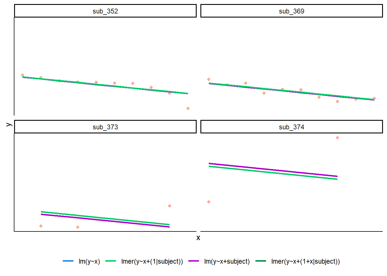
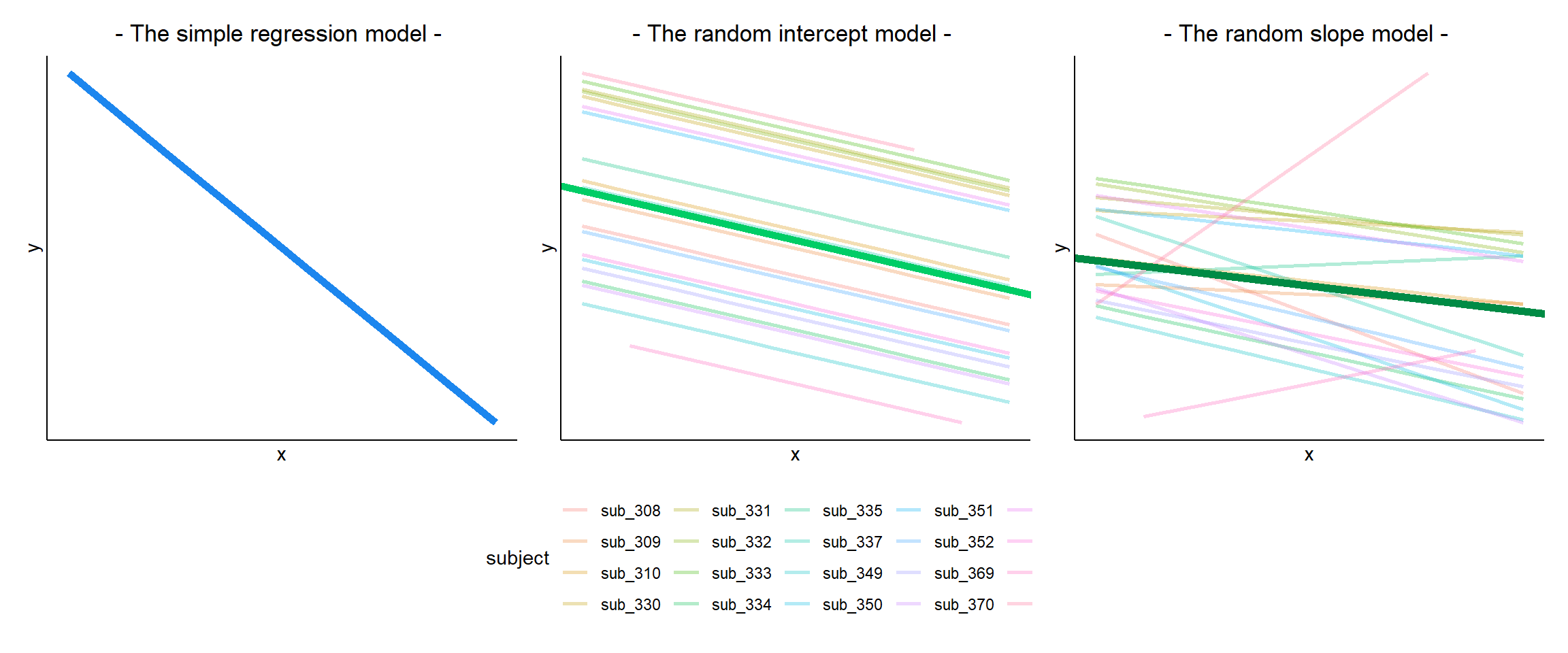
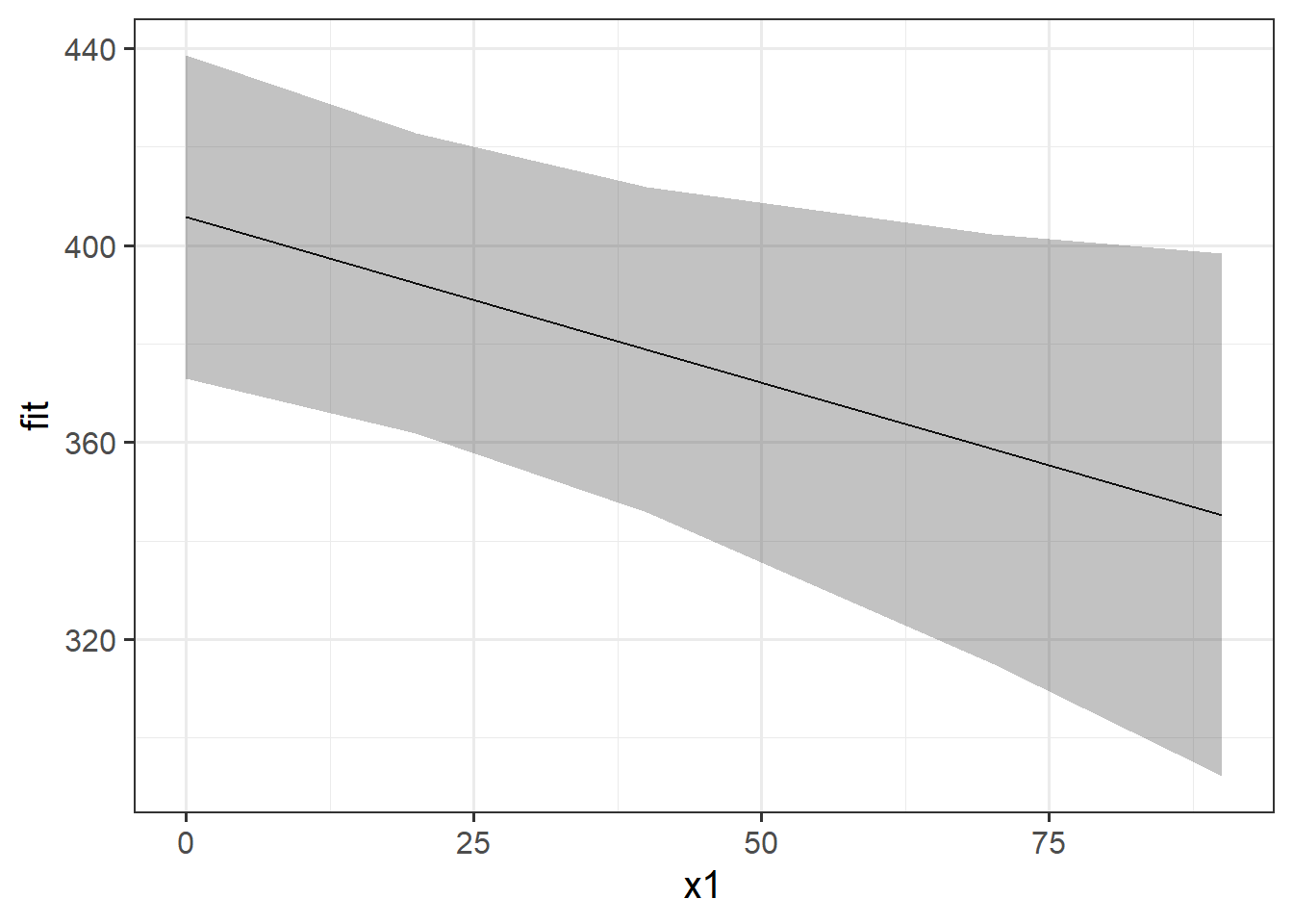
MLM allows us to model effects in the linear model as varying between groups. Our coefficients we remember from simple linear models (the $\beta$’s) are modelled as a distribution that has an overall mean around which our groups vary. We can see this in Figure 1, where both the intercept and the slope of the line are modelled as varying by-groups. Figure 1 shows the overall line in blue, with a given group’s line in green.

Figure 1: Multilevel Model. Each group (e.g. the group in the green line) deviates from the overall fixed effects (the blue line), and the individual observations (green points) deviate from their groups line

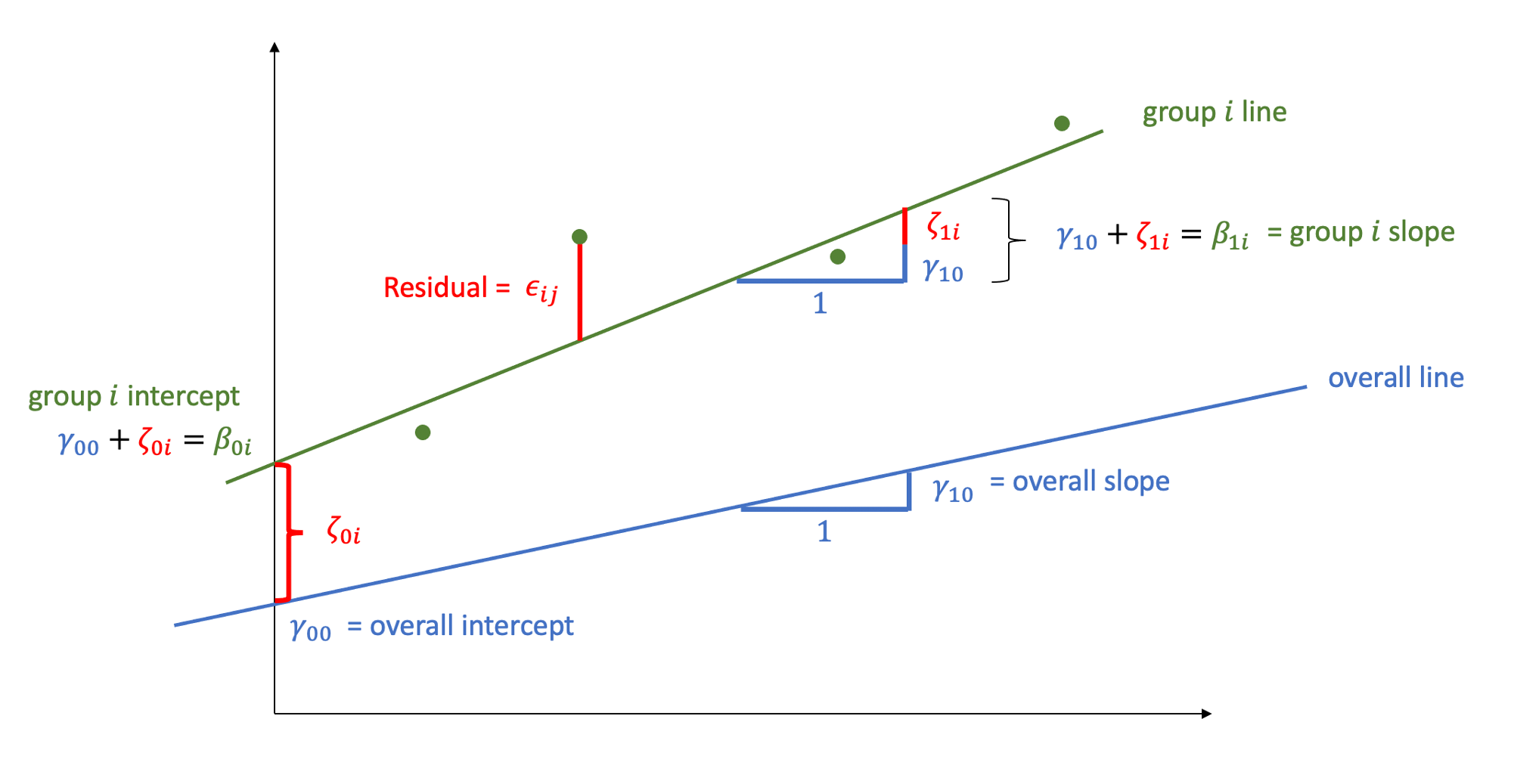
The formula notation for these models involves separating out our effects $\beta$ into two parts: the overall effect $\gamma$ + the group deviations ${\zeta }_i$:

$$\begin{array}{rl}& \text{for observation }j\text{ in group }i\\ \\ & \text{Level 1:}\\ & y_{ij}={\beta }_{0i}\cdot 1+{\beta }_{1i}\cdot x_{ij}+{\epsilon }_{ij}\\ & \text{Level 2:}\\ & {\beta }_{0i}={\gamma }_{00}+{\zeta }_{0i}\\ & {\beta }_{1i}={\gamma }_{10}+{\zeta }_{1i}\\ \\ & \text{Where:}\\ & {\gamma }_{00}\text{ is the population intercept, and }{\zeta }_{0i}\text{ is the deviation of group }i\text{ from }{\gamma }_{00}\\ & {\gamma }_{10}\text{ is the population slope, and }{\zeta }_{1i}\text{ is the deviation of group }i\text{ from }{\gamma }_{10}\end{array}$$

The group-specific deviations ${\zeta }_{0i}$ from the overall intercept are assumed to be normally distributed with mean $0$ and variance ${\sigma }_0^2$. Similarly, the deviations ${\zeta }_{1i}$ of the slope for group $i$ from the overall slope are assumed to come from a normal distribution with mean $0$ and variance ${\sigma }_1^2$. The correlation between random intercepts and slopes is $\rho =\text{Cor}({\zeta }_{0i},{\zeta }_{1i})=\frac{{\sigma }_{01}}{{\sigma }_0{\sigma }_1}$:

$$\left[\begin{array}{c}{\zeta }_{0i}\\ {\zeta }_{1i}\end{array}\right]\sim N(\left[\begin{array}{c}0\\ 0\end{array}\right],\left[\begin{array}{cc}{\sigma }_0^2& \rho {\sigma }_0{\sigma }_1\\ \rho {\sigma }_0{\sigma }_1& {\sigma }_1^2\end{array}\right])$$

The random errors, independently from the random effects, are assumed to be normally distributed with a mean of zero

$${ϵ}_{ij}\sim N(0,{\sigma }_{ϵ}^2)$$

MLM in R

We can fit these models using the R package lme4, and the function lmer(). Think of it like building your linear model lm(y ~ 1 + x), and then allowing effects (i.e. things on the right hand side of the ~ symbol) to vary by the grouping of your data. We specify these by adding (vary these effects | by these groups) to the model:

library(lme4)
m1 <- lmer(y ~ x + (1 + x | group), data = df)
summary(m1)

Linear mixed model fit by REML ['lmerMod']
Formula: y ~ x + (1 + x | group)
   Data: df

REML criterion at convergence: 637.9

Scaled residuals: 
     Min       1Q   Median       3Q      Max 
-2.49449 -0.57223 -0.01353  0.62544  2.39122 

Random effects:
 Groups   Name        Variance Std.Dev. Corr
 group    (Intercept) 2.2616   1.5038       
          x           0.7958   0.8921   0.55
 Residual             4.3672   2.0898       
Number of obs: 132, groups:  group, 20

Fixed effects:
            Estimate Std. Error t value
(Intercept)   1.7261     0.9673   1.785
x             1.1506     0.2968   3.877

Correlation of Fixed Effects:
  (Intr)
x -0.552

The summary of the lmer output returns estimated values for

Fixed effects:

• ${\hat{\gamma }}_{00}=1.726$
• ${\hat{\gamma }}_{10}=1.151$

Variability of random effects:

• ${\hat{\sigma }}_0=1.504$
• ${\hat{\sigma }}_1=0.892$

Correlation of random effects:

• $\hat{\rho }=0.546$

Residuals:

• ${\hat{\sigma }}_{ϵ}=2.09$

Flashcards: Getting p-values/CIs for Multilevel Models

Inference for multilevel models is tricky, and there are lots of different approaches.
You might find it helpful to think of the majority of these techniques as either:

A. Fitting a full model and a reduced model. These differ only with respect to the relevant effect. Comparing the overall fit of these models by some metric allows us to isolate the improvement due to our effect of interest. B. Fitting the full model and - using some method of approximating the degrees of freedom for the tests of whether a coefficient is zero. - constructing some confidence intervals (e.g. via bootstrapping) in order to gain a range of plausible values for the estimate (typically we then ask whether zero is within the interval)

Neither of these is correct or incorrect, but they each have different advantages. In brief:

• Satterthwaite $df$ = Very easy to implement, can fit with REML
• Kenward-Rogers $df$ = Good when working with small samples, can fit with REML
• Likelihood Ratio Tests = better with bigger samples (of groups, and of observations within groups), requires REML = FALSE
• Parametric Bootstrap = takes time to run, but in general a reliable approach. , requires REML = FALSE if doing comparisons, but not for confidence intervals
• Non-Parametric Bootstrap = takes time, needs careful thought about which levels to resample, but means we can relax distributional assumptions (e.g. about normality of residuals).

For the examples below, we’re investigating how “hours per week studied” influences a child’s reading age. We have data from 132 children from 20 schools, and we have fitted the model:

full_model <- lmer(reading_age ~ 1 + hrs_week + (1 + hrs_week | school), 
                   data = childread)

Use a normal approximation (not advisable)

Remember that the $t$ distribution starts to look more and more like the $z$ (“normal”) distribution when degrees of freedom increase? We could just assume we have infinite degrees of freedom in our test statistics, and pretend that the $t$-values we get are actually $z$-values. This is “anti-conservative” inasmuch as it is not a very cautious approach, and we are likely to have a higher false positive rate (e.g. more chance of saying “there is an effect!” when there actually isn’t.)

coefs <- as.data.frame(summary(full_model)$coefficients)
coefs$p.z <- 2 * (1 - pnorm(abs(coefs[,3])))
coefs

            Estimate Std. Error  t value          p.z
(Intercept) 1.726120  0.9672824 1.784504 0.0743417714
hrs_week    1.150637  0.2968219 3.876525 0.0001059589

Satterthwaite df approximation

There have been a couple of methods proposed to estimate the degrees of freedom in order to provide a better approximation to the null distribution of our tests. The way the Satterthwaite method has been implemented in R will just add a column for p-values to your summary(model) output).

Load the lmerTest package, refit the model, and voila!

library(lmerTest)
full_model <- lmer(reading_age ~ 1 + hrs_week + (1 + hrs_week | school), 
                   data = childread, REML = TRUE)
summary(full_model)$coefficients

            Estimate Std. Error       df  t value    Pr(>|t|)
(Intercept) 1.726120  0.9672824 16.23589 1.784504 0.093038229
hrs_week    1.150637  0.2968219 17.50762 3.876525 0.001155763

Reporting

To account for the extra uncertainty brought by the inclusion of random effects in the model, the degrees of freedom in the coefficients tests have been corrected via Satterthwaite’s method.
…
…
Weekly hours of reading practice was associated increased reading age ($\beta =1.15,SE=0.30,t({17.51}^{\ast })=3.88,p=.001$).

Note: if you have the lmerTest package loaded, then all the models you fit with lmer() will show p-values! If you want to stop this, then you will have to detach/unload the package, and refit the model.

detach("package:lmerTest", unload=TRUE)

Kenward Rogers df approximations

The Kenward-Rogers approach is slightly more conservative than the Satterthwaite method, and has been implemented for model comparison between a full model and a restricted model (a model without the parameter of interest), using the KR adjustment for the denominator degrees of freedom in the $F$-test.
For this, models must be fitted with REML, not ML. The function KRmodcomp() will take care of this and re-fit them for you.

library(pbkrtest)
restricted_model <- lmer(reading_age ~ 1 + (1 + hrs_week | school), 
                   data = childread, REML = TRUE)
full_model <- lmer(reading_age ~ 1 + hrs_week + (1 + hrs_week | school), 
                   data = childread, REML = TRUE)
KRmodcomp(full_model, restricted_model)

large : reading_age ~ 1 + hrs_week + (1 + hrs_week | school)
small : reading_age ~ 1 + (1 + hrs_week | school)
        stat    ndf    ddf F.scaling p.value   
Ftest 14.710  1.000 17.741         1 0.00124 **
---
Signif. codes:  0 '***' 0.001 '**' 0.01 '*' 0.05 '.' 0.1 ' ' 1

Reporting

To account for the extra uncertainty brought by the inclusion of random effects in the model, the denominator degrees of freedom in have been corrected via Kenward-Rogers’ method.
…
…
Inclusion of weekly hours of reading practice as a predictor was associated with an improvement in model fit ($F(1,{17.74}^{\ast })=14.71,p=.001$).

Likelihood Ratio Test (LRT)

Conduct a model comparison between your model and a restricted model (a model without the parameter of interest), evaluating the change in log-likelihood.

Likelihood

“likelihood” is a function that associates to a parameter the probability (or probability density) of observing the given sample data.
In simpler terms, the likelihood is the probability of the model given that we have this data.

The intuition behind likelihood:

1. I toss a coin 10 time and observed 8 Heads.
   
2. We can think of a ‘model’ of the process that governs the coin’s behaviour in terms of just one number: a parameter that indicates the probability of the coin landing on heads.
   I have two models:

• Model 1: The coin will land on heads 20% of the time. $P(Heads)=0.2$
  
• Model 2: The coin will land on heads 70% of the time. $P(Heads)=0.7$
  

3. Given the data I observe (see 1, above), we can (hopefully) intuit that Model 2 is more likely than Model 1.

For a (slightly) more detailed explanation, see here.

This method assumes that the ratio of two likelihoods will (as sample size increases) become closer to being ${\chi }^2$ distributed, and so may be unreliable for small samples.

Models must be fitted with ML, not REML. The function anova() will re-fit them for you.

restricted_model <- lmer(reading_age ~ 1 + (1 + hrs_week | school), 
                   data = childread, REML = FALSE)
full_model <- lmer(reading_age ~ 1 + hrs_week + (1 + hrs_week | school), 
                   data = childread, REML = FALSE)
anova(restricted_model, full_model, test = "Chisq")

Data: childread
Models:
restricted_model: reading_age ~ 1 + (1 + hrs_week | school)
full_model: reading_age ~ 1 + hrs_week + (1 + hrs_week | school)
                 npar    AIC    BIC  logLik deviance  Chisq Df Pr(>Chisq)    
restricted_model    5 660.52 674.93 -325.26   650.52                         
full_model          6 650.66 667.96 -319.33   638.66 11.857  1  0.0005744 ***
---
Signif. codes:  0 '***' 0.001 '**' 0.01 '*' 0.05 '.' 0.1 ' ' 1

Reporting

A likelihood ratio test indicated that the inclusion of weekly hours of reading practice as a predictor was associated with an improvement in model fit (${\chi }^2(1)=11.86,p<.001$).

Parametric Bootstrap LRT

There are also various “bootstrapping” methods which it is worth looking into. Think back to USMR when we first learned about hypothesis testing. Remember that we did lots of simulating data, so that we can compare what we actually observe with what we would expect if the null hypothesis were true? By doing this, we were essentially creating a null distribution, so that our calculating a p-value can become an issue of summarising data (e.g. calculate the proportion of our simulated null distribution that is more extreme than our observed statistic)

Instead of assuming that the likelihood ratio test statistics are ${\chi }^2$-distributed, we can bootstrap this test instead. This approach simulates data from the simpler model, fits both the simple model and the complex model and evaluates the change in log-likelihood. By doing this over and over again, we build a distribution of what changes in log-likelihood we would be likely to see if the more complex model is not any better. In this way it actually constructs a distribution reflecting our null hypothesis, against which we can then compare our actual observed effect

library(pbkrtest)
restricted_model <- lmer(reading_age ~ 1 + (1 + hrs_week | school), 
                   data = childread, REML = FALSE)
full_model <- lmer(reading_age ~ 1 + hrs_week + (1 + hrs_week | school), 
                   data = childread, REML = FALSE)
PBmodcomp(full_model, restricted_model, nsim=1000)

Reporting

A parametric bootstrap likelihood ratio test (R = 1000) indicated that the inclusion of weekly hours of reading practice as a predictor was associated with an improvement in model fit ($LRT=11.84,p=.002$).

Parametric Bootstrap Confidence Intervals

Much the same as above, but with just one model we simulate data many times and refit the model, so that we get an empirical distribution that we can use to construct confidence intervals for our effects.

full_model <- lmer(reading_age ~ 1 + hrs_week + (1 + hrs_week | school), 
                   data = childread, REML = TRUE)
confint(full_model, method="boot")

                 2.5 %   97.5 %
.sig01       0.0000000 3.913368
.sig02      -0.5647829 1.000000
.sig03       0.3927015 1.376779
.sigma       1.7921405 2.349858
(Intercept) -0.1214629 3.370657
hrs_week     0.5567827 1.752359

Reporting

95% Confidence Intervals were obtained via parametric bootstrapping with 1000 iterations.
…
…
Weekly hours of reading practice was associated increased reading age ($\beta =1.15,95$).

Non-Parametric Bootstrap Confidence Intervals

It’s worth noting that there are many different types of bootstrapping that we can conduct. Different methods of bootstrapping vary with respect to the assumptions we will have to make when using them for drawing inferences. For instance, the parametric bootstrap discussed above assumes that explanatory variables are fixed and that model specification and the distributions such as ${\zeta }_i\sim N(0,{\sigma }_{\zeta })$ and ${\epsilon }_i\sim N(0,{\sigma }_{\epsilon })$ are correct.
An alternative is to generate a distribution by resampling with replacement from our data, fitting our model to the resample, and then repeating this over and over. This doesn’t have to rely on assumptions about the shape of the distributions of ${\zeta }_i$ and ${\epsilon }_i$ - we just need to ensure that we correctly specify the hierarchical dependency of data. It does, however, require the decision of at which levels to resample.

full_model <- lmer(reading_age ~ 1 + hrs_week + (1 + hrs_week | school), 
                   data = childread, REML = TRUE)
library(lmeresampler)
fullmod_bs <- 
  bootstrap(full_model, # this is the model
            .f = fixef, # we want the fixef from each bootstrap
            type = "case", # case based bootstrap
            B=2000, # do 2000 bootstraps
            resample = c(TRUE, TRUE) # resample both schools and individual children
  ) 
confint(fullmod_bs, type = "perc")

# A tibble: 2 × 6
  term        estimate  lower upper type  level
  <chr>          <dbl>  <dbl> <dbl> <chr> <dbl>
1 (Intercept)     1.73 -1.44   3.57 perc   0.95
2 hrs_week        1.15  0.681  2.02 perc   0.95

Reporting

95% Confidence Intervals were obtained via case-based bootstrapping (resampling both toy types and individual toys) with 2000 iterations.
…
…
Weekly hours of reading practice was associated increased reading age ($\beta$ = 1.1506375, 95% CI [0.6811553 – 2.0204023]).