| variable | description |
|---|---|
| ppt | Participant ID |
| name | Participant Name |
| laa | Local Authority Area |
| outdoor_time | Self report estimated number of hours per week spent outdoors |
| wellbeing | Warwick-Edinburgh Mental Wellbeing Scale (WEMWBS), a self-report measure of mental health and well-being. The scale is scored by summing responses to each item, with items answered on a 1 to 5 Likert scale. The minimum scale score is 14 and the maximum is 70. |
| density | LAA Population Density (people per square km) |
Assumptions, Diagnostics, and Random Effect Structures
Preliminaries
- Create a new RMarkdown document or R script (whichever you like) for this week.
Exercises: Assumptions & Diagnostics
For these next set of exercises we will return to our study from Week 1, in which researchers want to study the relationship between time spent outdoors and mental wellbeing, across all of Scotland. Data is collected from 20 of the Local Authority Areas and is accessible at https://uoepsy.github.io/data/LAAwellbeing.csv.
Question 1
The code below will read in the data and fit the model with by-LAA random intercepts and slopes of outdoor time.
library(tidyverse)
library(lme4)
scotmw <- read_csv("https://uoepsy.github.io/data/LAAwellbeing.csv")
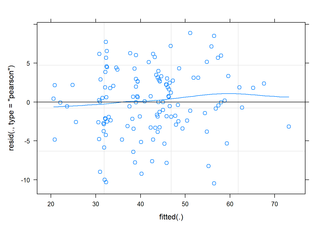
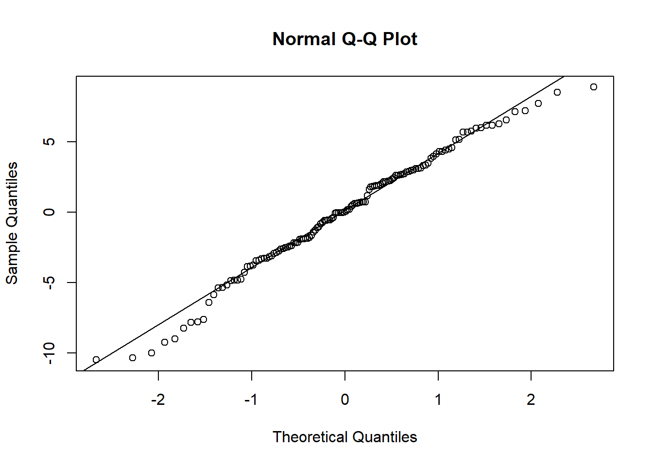
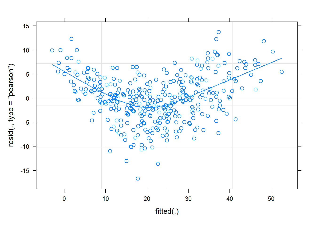
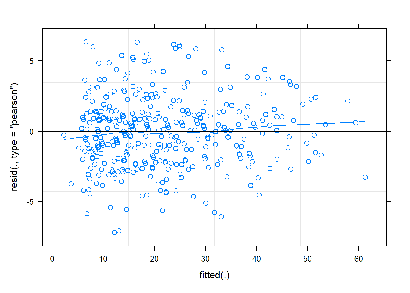
rs_model <- lmer(wellbeing ~ 1 + outdoor_time + (1 + outdoor_time | laa), data = scotmw)- Plot the residuals vs fitted model, and assess the extend to which the assumption holds that the residuals are zero mean.
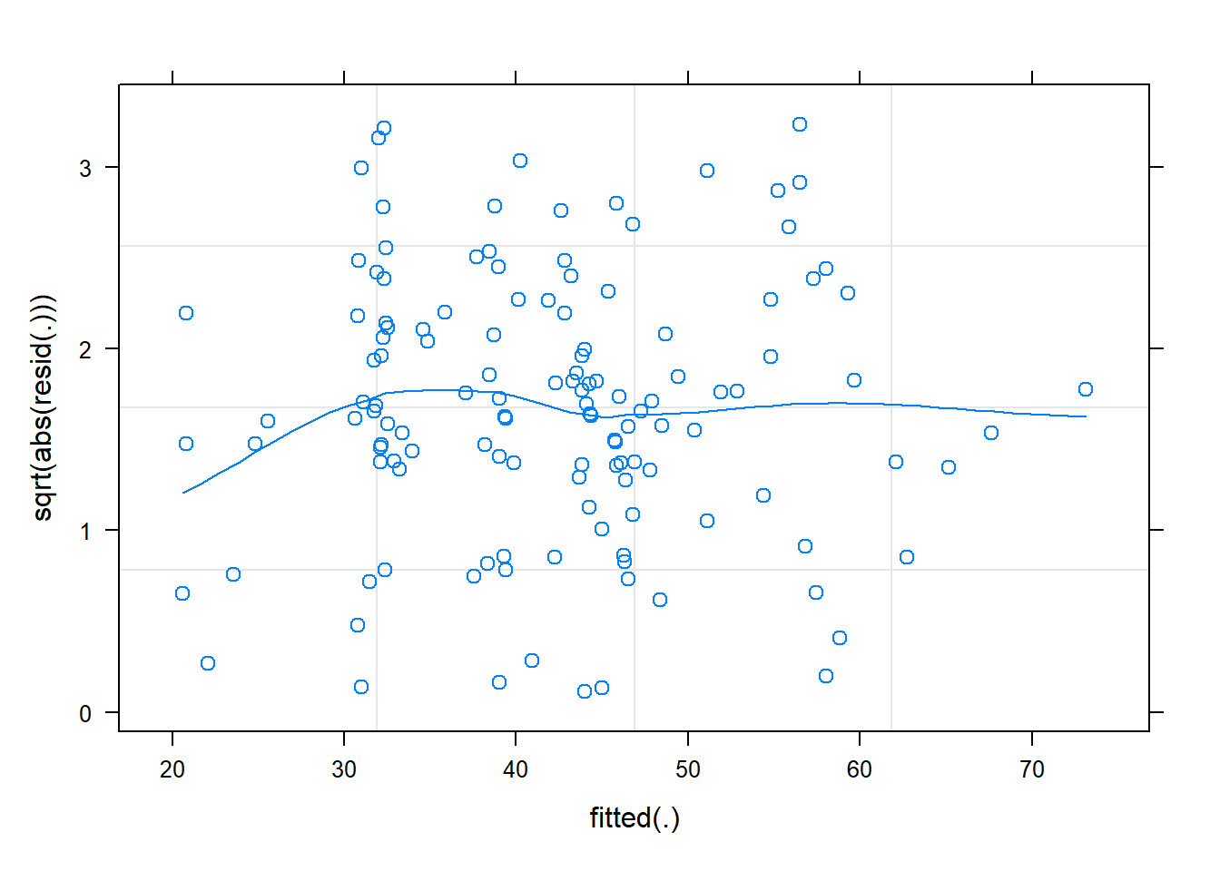
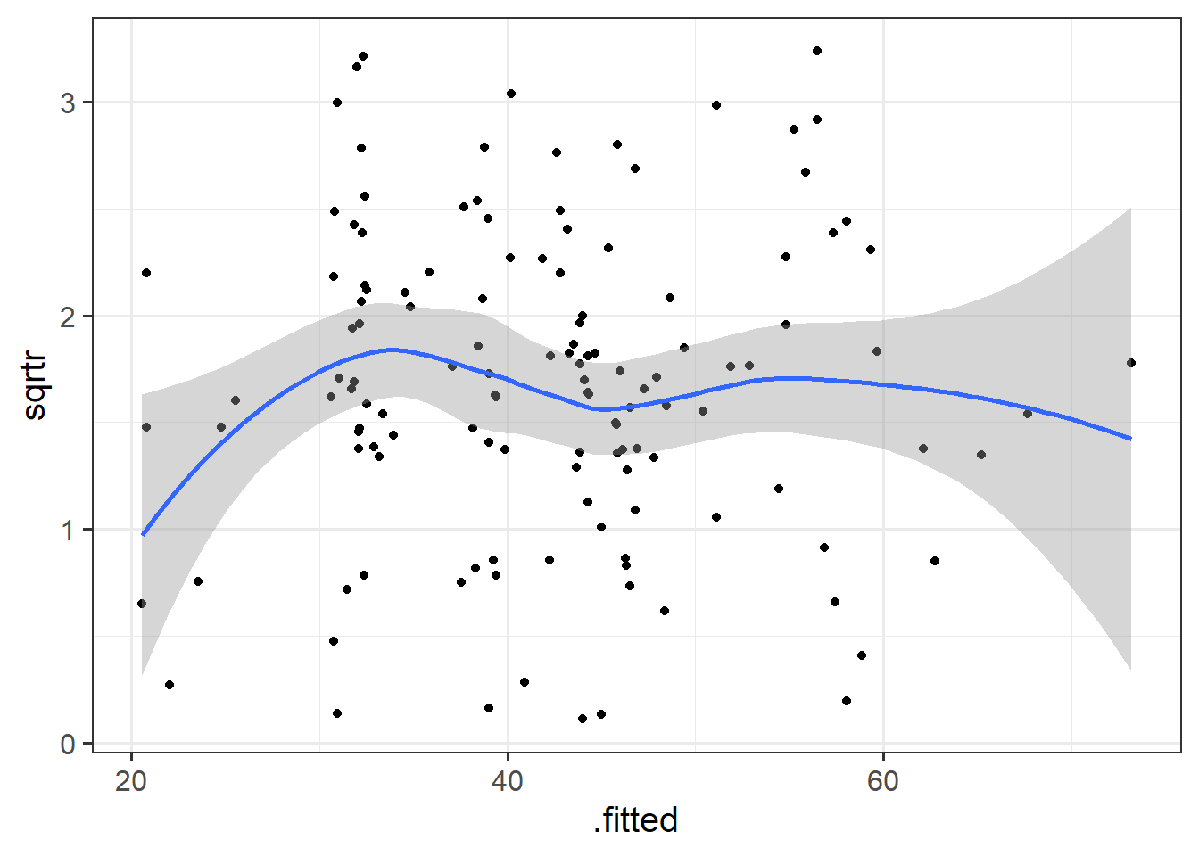
- Construct a scale-location plot. This is where the square-root of the absolute value of the standardised residuals is plotted against the fitted values, and allows you to more easily assess the assumption of constant variance.
- Optional: can you create the same plot using ggplot, starting with the
augment()function from the broom.mixed package?
Hint: plot(model) will give you this plot, but you might want to play with the type = c(......) argument to get the smoothing line
Question 2
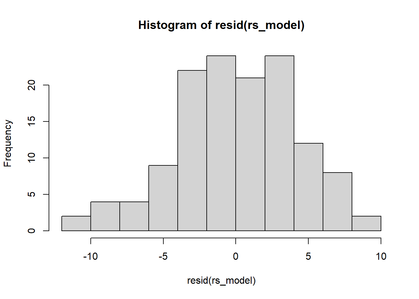
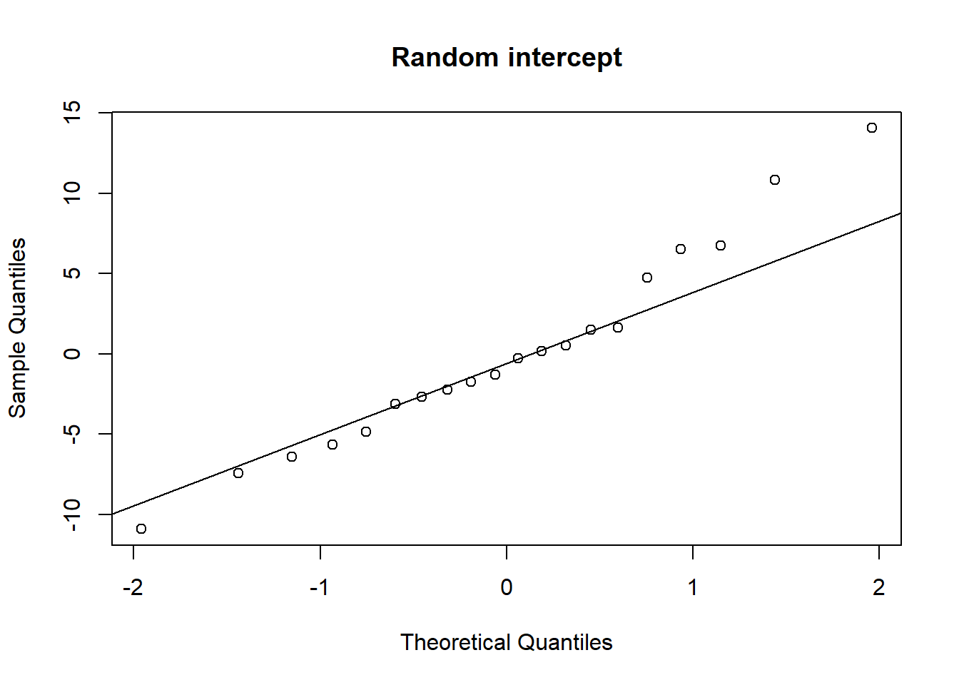
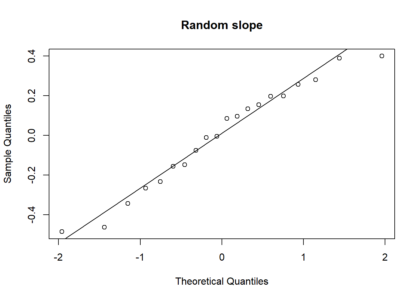
Examine the normality of both the level 1 and level 2 residuals.
Hints:
- Use
hist()if you like, orqqnorm(residuals)followed byqqline(residuals) - Extracting the level 2 residuals (the random effects) can be difficult.
ranef(model)will get you some of the way.
Question 3
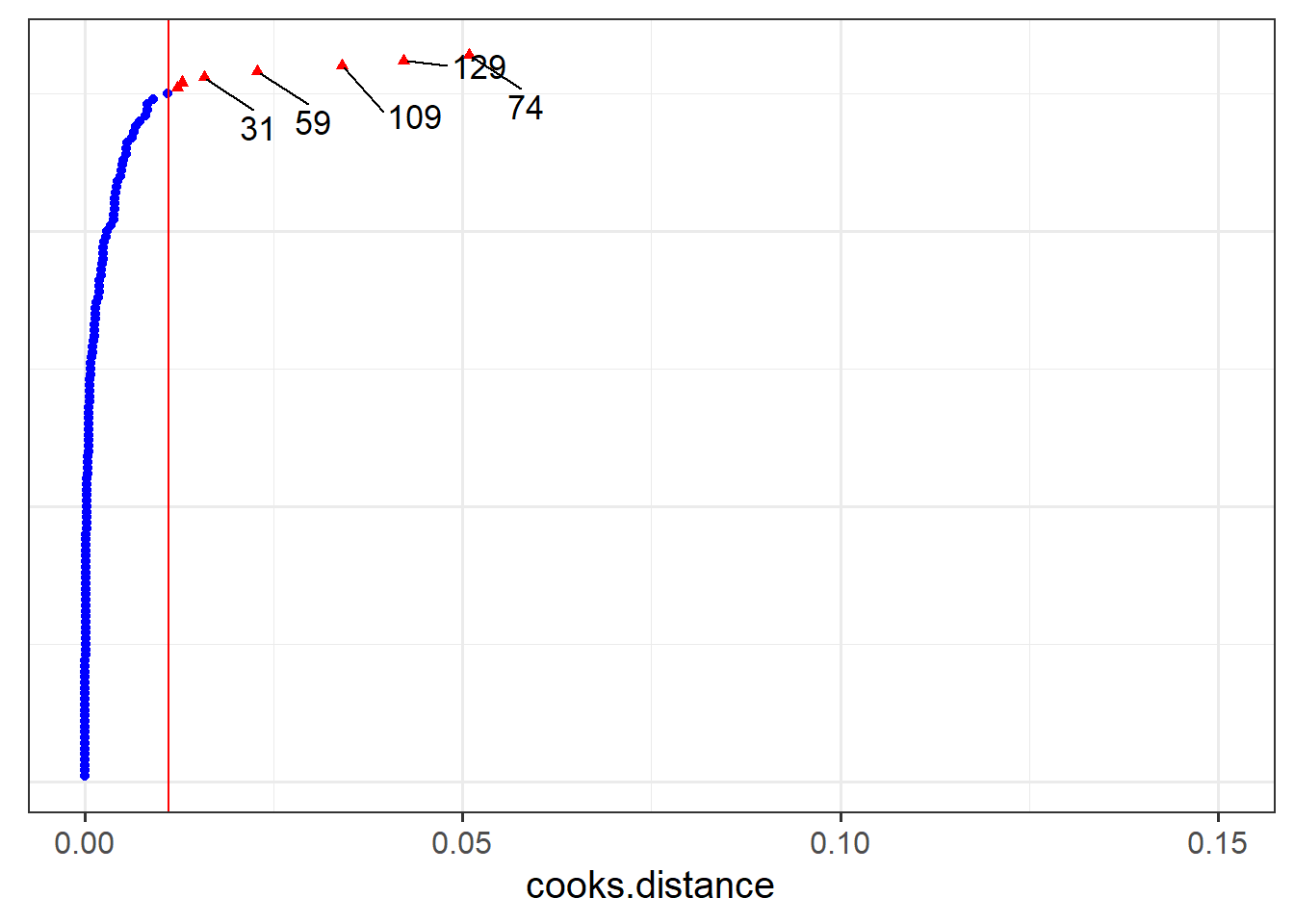
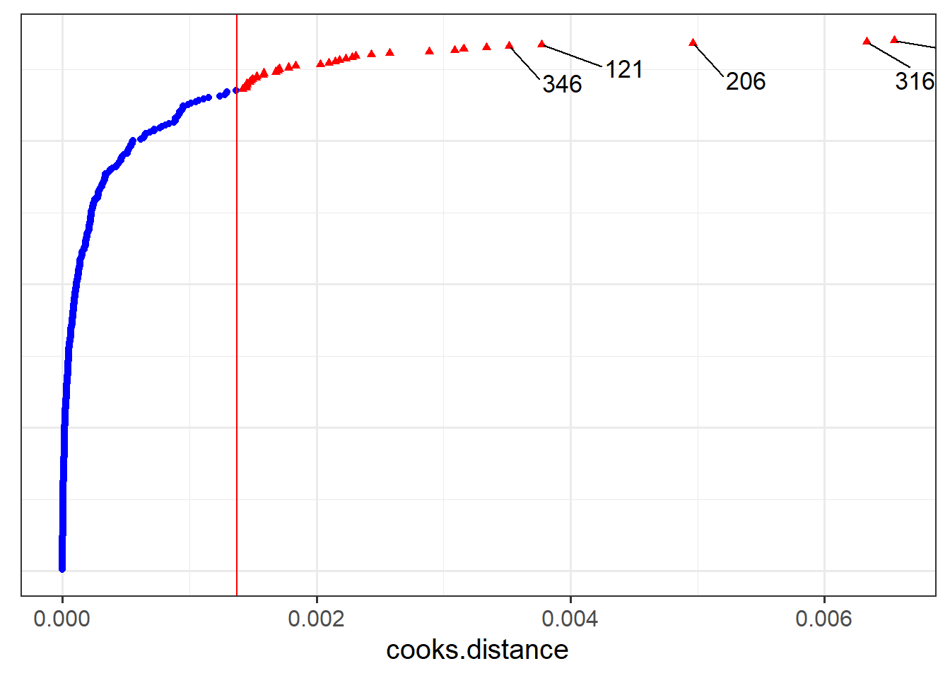
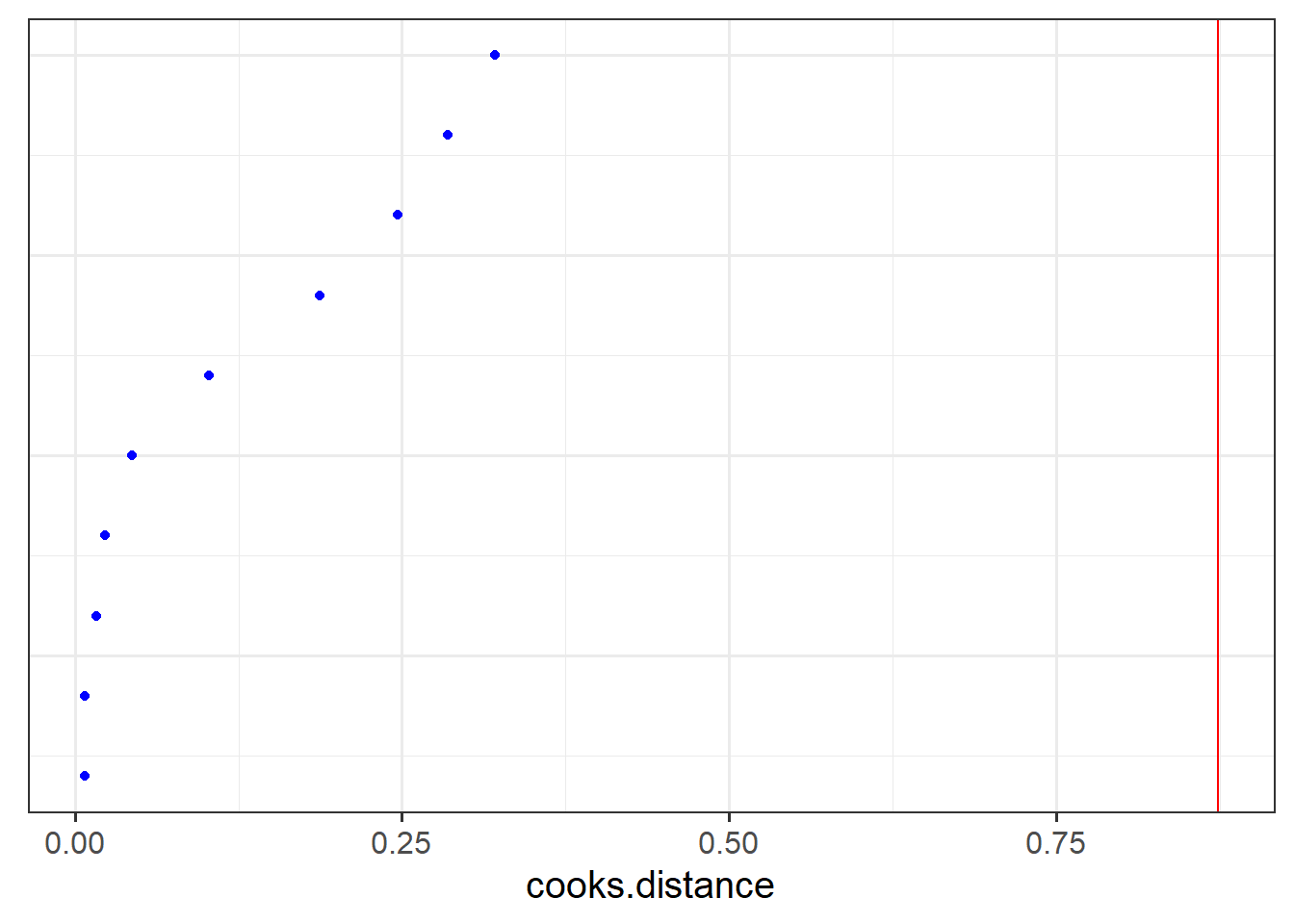
- Which person in the dataset has the greatest influence on our model?
- For which person is the model fit the worst (i.e., who has the highest residual?)
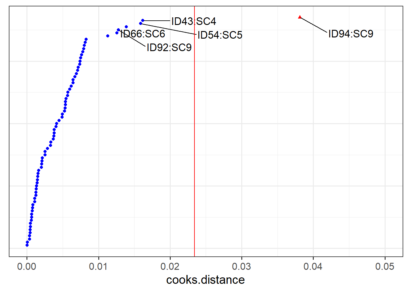
- Which LAA has the greatest influence on our model?
Hints:
- as well as
hlm_influence()in the HLMdiag package there is another nice function,hlm_augment() - we can often end up in confusion because the \(i^{th}\) observation inputted to our model (and therefore the \(i^{th}\) observation of
hlm_influence()output) might not be the \(i^{th}\) observation in our original dataset - there may be missing data! (Luckily, we have no missing data in this dataset).

Question 4
- Looking at the random effects, which LAA shows the least improvement in wellbeing as outdoor time increases, and which shows the greatest improvement?
- What is the estimated wellbeing for people from City of Edinburgh with zero hours of outdoor time per week, and what is their associated increases in wellbeing for every hour per week increase in outdoor time?
Random Effect Structures
Random effect structures can get pretty complicated quite quickly. Very often it is not the random effects part that is of specific interest to us, but we wish to estimate random effects in order to more accurately partition up the variance in our outcome variable and provide better estimates of fixed effects.
It is a fine balance between fitting the most sophisticated model structure that we possibly can, and fitting a model that converges without too much simplification. Typically for many research designs, the following steps will keep you mostly on track to finding the maximal model:
lmer(outcome ~ fixed effects + (random effects | grouping structure))
Specify the
outcome ~ fixed effectsbit first.- The outcome variable should be clear: it is the variable we are wishing to explain/predict.
- The fixed effects are the things we want to use to explain/predict variation in the outcome variable. These will often be the things that are of specific inferential interest, and other covariates. Just like the simple linear model.
If there is a grouping structure to your data, and those groups (preferably n>5) are perceived as a random sample of a wider population (the specific groups aren’t interesting to you), then consider fitting them in the random effects part
(1 | grouping).If any of the things in the fixed effects vary within the groups, it might be possible to also include them as random effects.
- as a general rule, don’t specify random effects that are not also specified as fixed effects (an exception could be specifically for model comparison, to isolate the contribution of the fixed effect).
- For things that do not vary within the groups, it rarely makes sense to include them as random effects. For instance if we had a model with
lmer(score ~ genetic_status + (1 + genetic_status | participant))then we would be trying to model a process where “the effect of genetic_status on scores is different for each participant”. But if you consider an individual participant, their genetic status never changes. For participant \(i\), what is “the effect of genetic status on score”? It’s undefined. This is because genetic status only varies between participants.
- as a general rule, don’t specify random effects that are not also specified as fixed effects (an exception could be specifically for model comparison, to isolate the contribution of the fixed effect).
Random Effects in lme4
Below are a selection of different formulas for specifying different random effect structures, taken from the lme4 vignette. This might look like a lot, but over time and repeated use of multilevel models you will get used to reading these in a similar way to getting used to reading the formula structure of y ~ x1 + x2 in all our linear models.
| Formula | Alternative | Meaning |
|---|---|---|
| \(\text{(1 | g)}\) | \(\text{1 + (1 | g)}\) | Random intercept with fixed mean |
| \(\text{(1 | g1/g2)}\) | \(\text{(1 | g1) + (1 | g1:g2)}\) | Intercept varying among \(g1\) and \(g2\) within \(g1\) |
| \(\text{(1 | g1) + (1 | g2)}\) | \(\text{1 + (1 | g1) + (1 | g2)}\) | Intercept varying among \(g1\) and \(g2\) |
| \(\text{x + (x | g)}\) | \(\text{1 + x + (1 + x | g)}\) | Correlated random intercept and slope |
| \(\text{x + (x || g)}\) | \(\text{1 + x + (x | g) + (0 + x | g)}\) | Uncorrelated random intercept and slope |
Table 1: Examples of the right-hand-sides of mixed effects model formulas. \(g\), \(g1\), \(g2\) are grouping factors, \(x\) is a predictor variable.
Convergence Issues and What To Do
Singular fits
You may have noticed that some of our models over the last few weeks have been giving a warning: boundary (singular) fit: see ?isSingular.
Up to now, we’ve been largely ignoring these warnings. However, this week we’re going to look at how to deal with this issue.
boundary (singular) fit: see ?isSingular
The warning is telling us that our model has resulted in a ‘singular fit’. Singular fits often indicate that the model is ‘overfitted’ - that is, the random effects structure which we have specified is too complex to be supported by the data.
Perhaps the most intuitive advice would be remove the most complex part of the random effects structure (i.e. random slopes). This leads to a simpler model that is not over-fitted. In other words, start simplying from the top (where the most complexity is) to the bottom (where the lowest complexity is). Additionally, when variance estimates are very low for a specific random effect term, this indicates that the model is not estimating this parameter to differ much between the levels of your grouping variable. It might, in some experimental designs, be perfectly acceptable to remove this or simply include it as a fixed effect.
A key point here is that when fitting a mixed model, we should think about how the data are generated. Asking yourself questions such as “do we have good reason to assume subjects might vary over time, or to assume that they will have different starting points (i.e., different intercepts)?” can help you in specifying your random effect structure
You can read in depth about what this means by reading the help documentation for ?isSingular. For our purposes, a relevant section is copied below:
… intercept-only models, or 2-dimensional random effects such as intercept + slope models, singularity is relatively easy to detect because it leads to random-effect variance estimates of (nearly) zero, or estimates of correlations that are (almost) exactly -1 or 1.
Convergence warnings
Issues of non-convergence can be caused by many things. If you’re model doesn’t converge, it does not necessarily mean the fit is incorrect, however it is is cause for concern, and should be addressed, else you may end up reporting inferences which do not hold.
There are lots of different things which you could do which might help your model to converge. A select few are detailed below:
double-check the model specification and the data
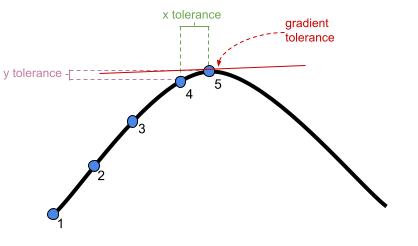
adjust stopping (convergence) tolerances for the nonlinear optimizer, using the optCtrl argument to [g]lmerControl. (see
?convergencefor convergence controls).- What is “tolerance”? Remember that our optimizer is the the method by which the computer finds the best fitting model, by iteratively assessing and trying to maximise the likelihood (or minimise the loss).
center and scale continuous predictor variables (e.g. with
scale)Change the optimization method (for example, here we change it to
bobyqa):lmer(..., control = lmerControl(optimizer="bobyqa"))
glmer(..., control = glmerControl(optimizer="bobyqa"))Increase the number of optimization steps:
lmer(..., control = lmerControl(optimizer="bobyqa", optCtrl=list(maxfun=50000))
glmer(..., control = glmerControl(optimizer="bobyqa", optCtrl=list(maxfun=50000))Use
allFit()to try the fit with all available optimizers. This will of course be slow, but is considered ‘the gold standard’; “if all optimizers converge to values that are practically equivalent, then we would consider the convergence warnings to be false positives.”Consider simplifying your model, for example by removing random effects with the smallest variance (but be careful to not simplify more than necessary, and ensure that your write up details these changes)
Exercises: Random Effect Structures
Crossed Ranefs
Data: Test-enhanced learning
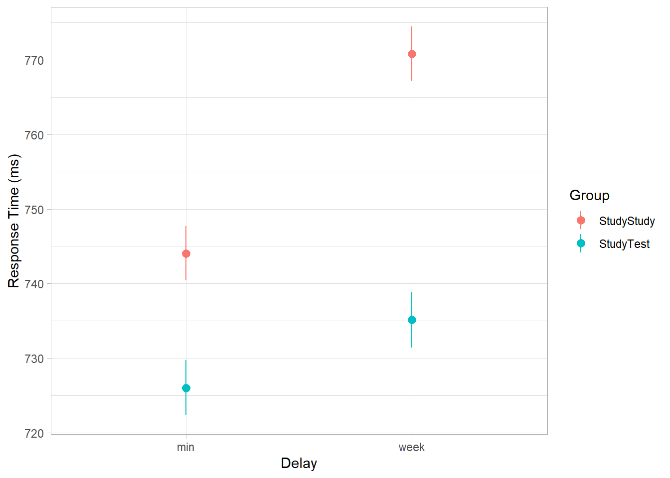
An experiment was run to conceptually replicate “test-enhanced learning” (Roediger & Karpicke, 2006): two groups of 25 participants were presented with material to learn. One group studied the material twice (StudyStudy), the other group studied the material once then did a test (StudyTest). Recall was tested immediately (one minute) after the learning session and one week later. The recall tests were composed of 175 items identified by a keyword (Test_word). One of the researchers’ questions concerned how test-enhanced learning influences time-to-recall.
The critical (replication) prediction is that the StudyStudy group should perform somewhat better on the immediate recall test, but the StudyTest group will retain the material better and thus perform better on the 1-week follow-up test.
| variable | description |
|---|---|
| Subject_ID | Unique Participant Identifier |
| Group | Group denoting whether the participant studied the material twice (StudyStudy), or studied it once then did a test (StudyTest) |
| Delay | Time of recall test ('min' = Immediate, 'week' = One week later) |
| Test_word | Word being recalled (175 different test words) |
| Correct | Whether or not the word was correctly recalled |
| Rtime | Time to recall word (milliseconds) |
The following code loads the data into your R environment by creating a variable called tel:
load(url("https://uoepsy.github.io/data/testenhancedlearning.RData"))
Question 5
Load and plot the data.
For this week, we’ll use Reaction Time as our proxy for the test performance, so you’ll probably want that variable on the y-axis.
Does it look like the effect was replicated?
Question 6
The critical (replication) prediction is that the
StudyStudygroup should perform somewhat better on the immediate recall test, but theStudyTestgroup will retain the material better and thus perform better on the 1-week follow-up test.
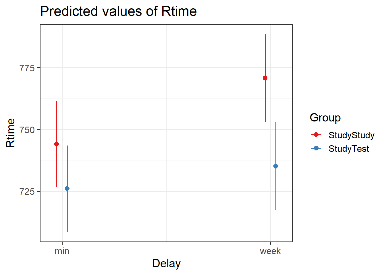
Test the critical hypothesis using a multi-level model.
Try to fit the maximally complex random effect structure that is supported by the experimental design.
NOTE: Your model probably won’t converge. We’ll deal with that in the next question
Hints:
- We can expect variability across subjects (some people are better at learning than others) and across items (some of the recall items are harder than others). How should this be represented in the random effects?
- If a model takes ages to fit, you might want to cancel it by pressing the escape key. It is normal for complex models to take time, but for the purposes of this task, give up after a couple of minutes, and try simplifying your model.
Question 7
Often, models with maximal random effect structures will not converge, or will obtain a singular fit. One suggested approach here is to simplify the model until you achieve convergence (Barr et al., 2013).
Incrementally simplify your model from the previous question until you obtain a model that converges and is not a singular fit.
Hint: you can look at the variance estimates and correlations easily by using the VarCorr() function. What jumps out?
Nested Random Effects
Data: Naming
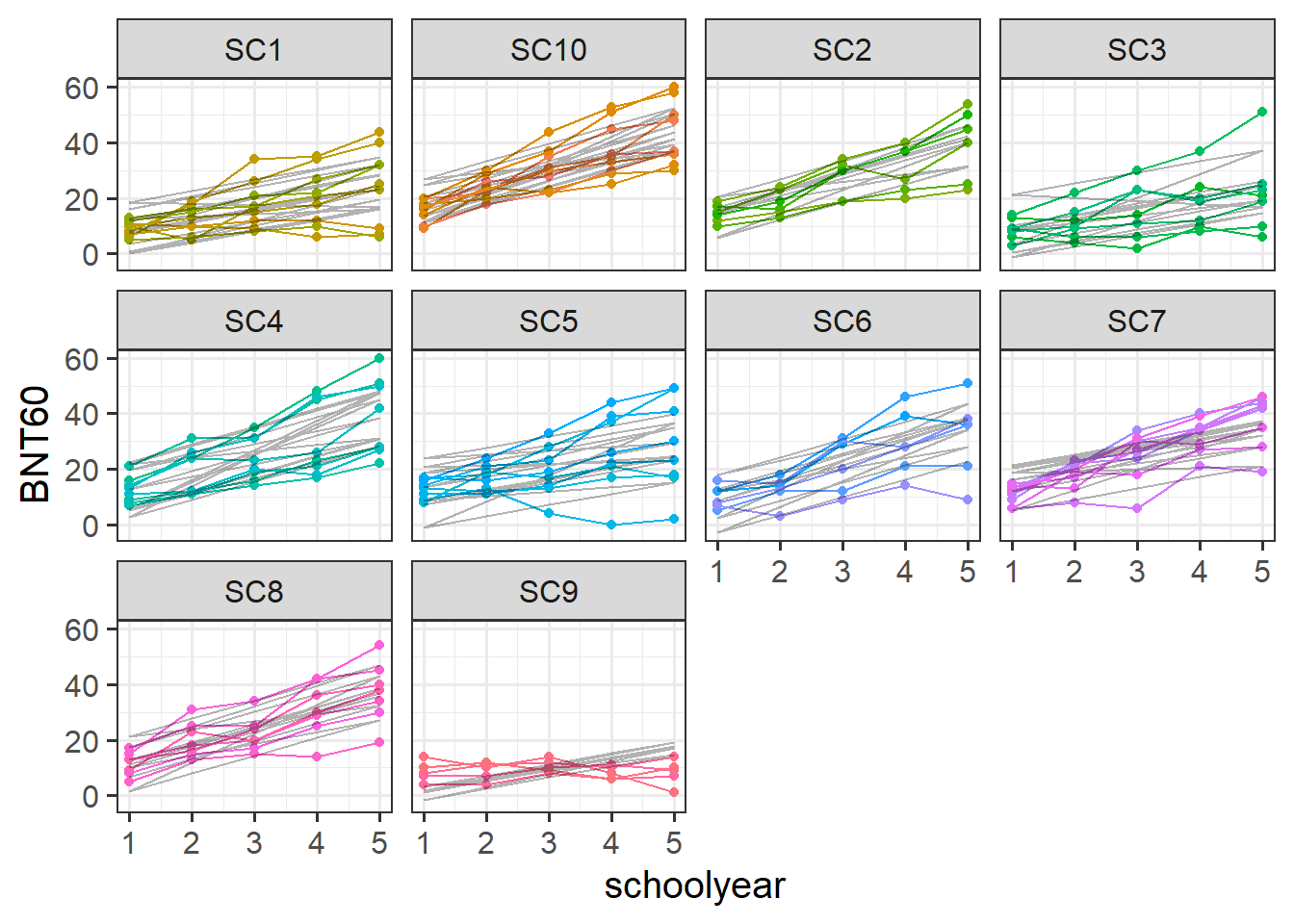
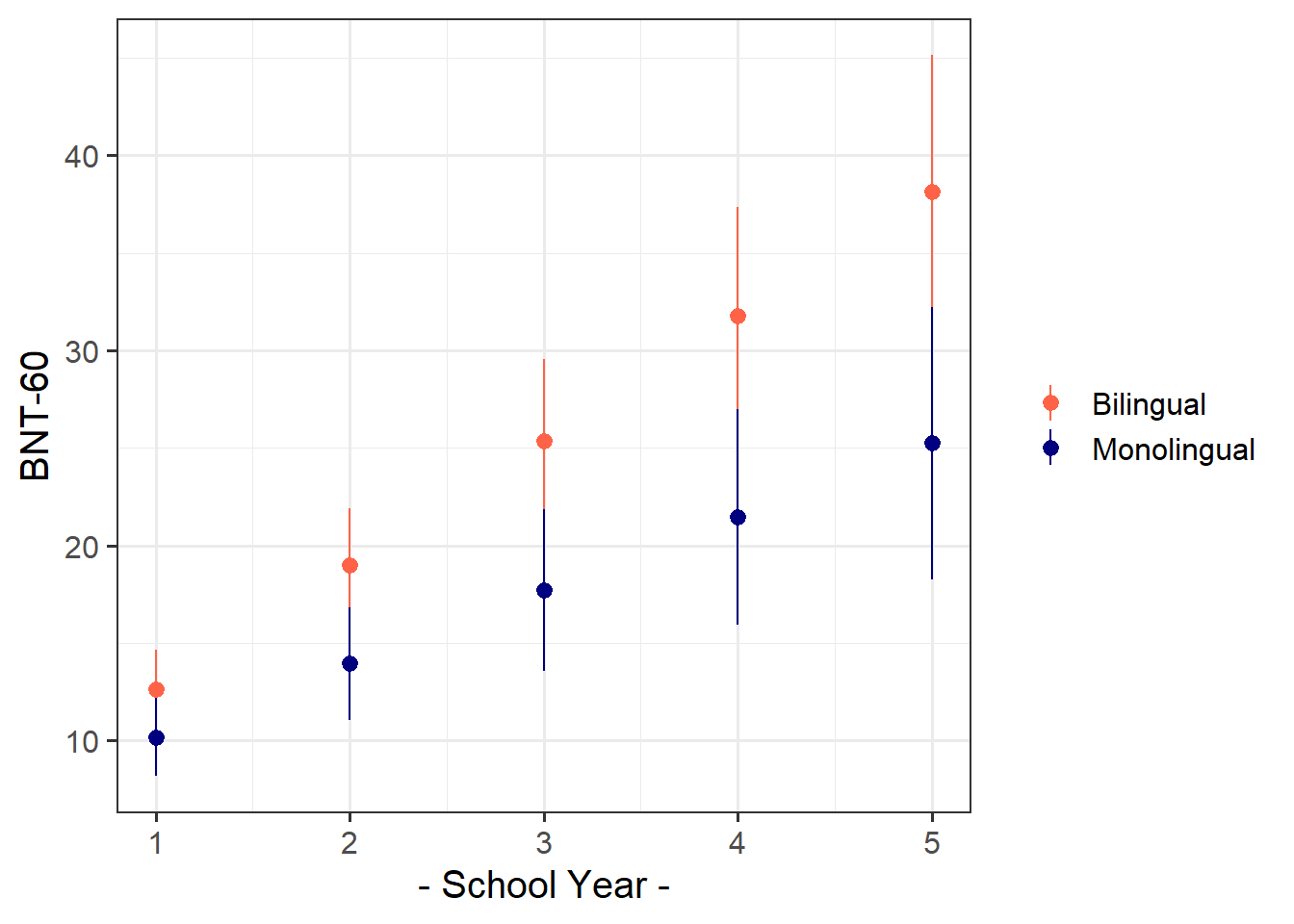
74 children from 10 schools were administered the full Boston Naming Test (BNT-60) on a yearly basis for 5 years to examine development of word retrieval. Five of the schools taught lessons in a bilingual setting with English as one of the languages, and the remaining five schools taught in monolingual English.
The data is available at https://uoepsy.github.io/data/bntmono.csv.
| variable | description |
|---|---|
| child_id | unique child identifier |
| school_id | unique school identifier |
| BNT60 | score on the Boston Naming Test-60. Scores range from 0 to 60 |
| schoolyear | Year of school |
| mlhome | Mono/Bi-lingual School. 0 = Bilingual, 1 = Monolingual |
Question 8
Let’s start by thinking about our clustering - we’d like to know how much of the variance in BNT60 scores is due to the clustering of data within children, who are themselves within schools. One easy way of assessing this is to fit an intercept only model, which has the appropriate random effect structure.
Using the model below, calculate the proportion of variance attributable to the clustering of data within children within schools.
bnt_null <- lmer(BNT60 ~ 1 + (1 | school_id/child_id), data = bnt)Hint: the random intercept variances are the building blocks here. There are no predictors in this model, so all the variance in the outcome gets attributed to either school-level nesting, child-level nesting, or else is lumped into the residual.
Question 9
Fit a model examining the interaction between the effects of school year and mono/bilingual teaching on word retrieval, with random intercepts only for children and schools.
Hint: make sure your variables are of the right type first - e.g. numeric, factor etc
Examine the fit and consider your model assumptions, and assess what might be done to improve the model in order to make better statistical inferences.
Question 10
Using a method of your choosing, conduct inferences (i.e. obtain p-values or confidence intervals) from your final model and write up the results.
Footnotes
It’s always going to be debateable about what is ‘too high’ because in certain situations you might expect correlations close to 1. It’s best to think through whether it is a feasible value given the study itself↩︎