Principal Component Analysis (PCA)

Relevant packages

• psych

Thinking about measurement

Take a moment to think about the various constructs that you are often interested in as a researcher. This might be anything from personality traits, to language proficiency, social identity, anxiety etc. How we measure such constructs is a very important consideration for research. The things we’re interested in are very rarely the things we are directly measuring.

Consider how we might assess levels of anxiety or depression. Can we ever directly measure anxiety? ¹. More often than not, we measure these things using questionnaire based methods, to capture the multiple dimensions of the thing we are trying to assess. Twenty questions all measuring different aspects of anxiety are (we hope) going to correlate with one another if they are capturing some commonality (the construct of “anxiety”). But they introduce a problem for us, which is how to deal with 20 variables that represent (in broad terms) the same thing. How can we assess “effects on anxiety”, rather than “effects on anxiety q1”, “effects on anxiety q2”, …, etc.

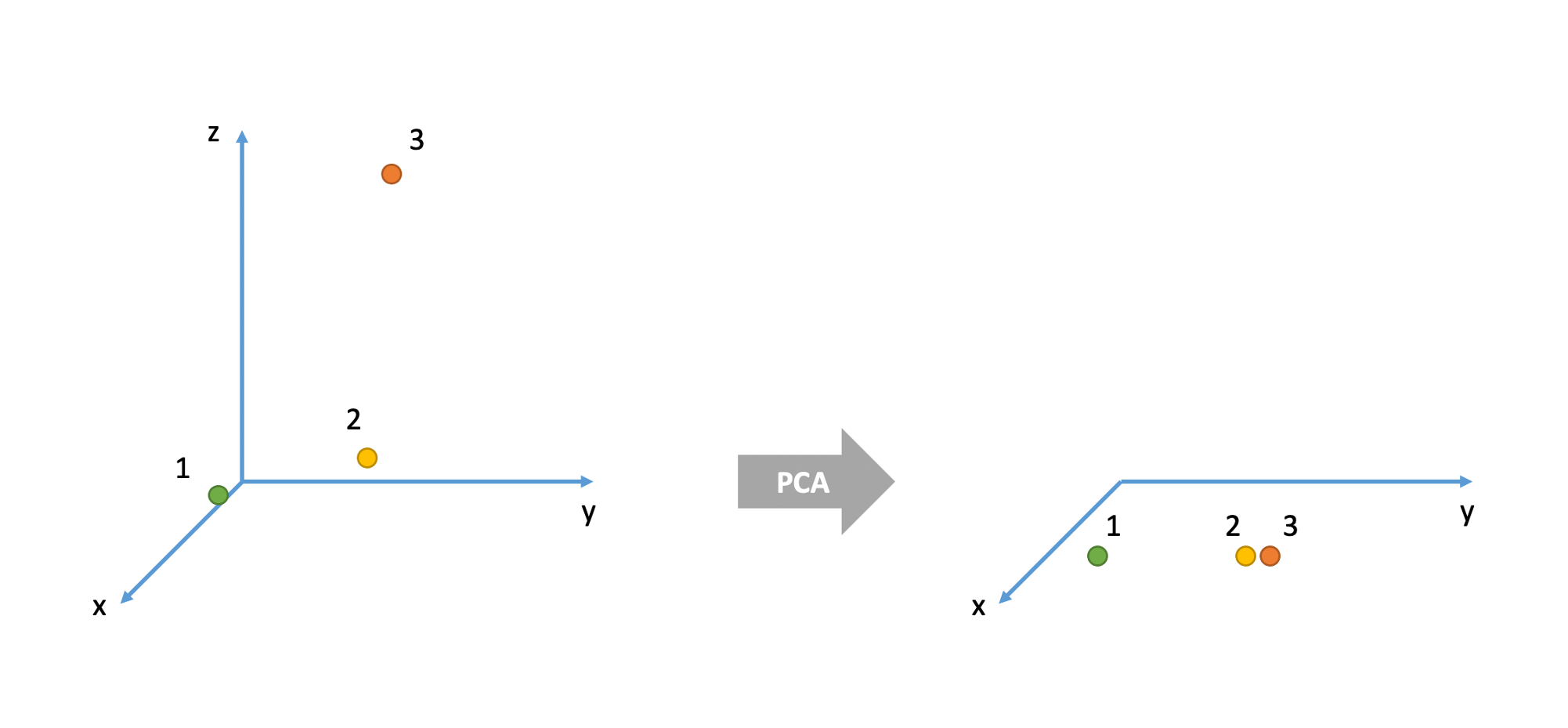
This leads us to the idea of reducing the dimensionality of our data. Can we capture a reasonable amount of the information from our 20 questions in a smaller number of variables?

The goal of principal component analysis (PCA) is to find a smaller number of uncorrelated variables which are linear combinations of the original ( many ) variables and explain most of the variation in the data.

Exercises: Police Performance

Data: Police Performance

The file police_performance.csv (available at https://uoepsy.github.io/data/police_performance.csv) contains data on fifty police officers who were rated in six different categories as part of an HR procedure. The rated skills were:

• communication skills: commun
• problem solving: probl_solv
• logical ability: logical
• learning ability: learn
• physical ability: physical
• appearance: appearance

The data also contains information on each police officer’s arrest rate (proportion of arrests that lead to criminal charges).

We are interested in if the skills ratings by HR are a good set of predictors of police officer success (as indicated by their arrest rate).

1. Explore

First things first, we should always plot and describe our data. This is always a sensible thing to do - while many of the datasets we give you are nice and clean and organised, the data you get out of questionnaire tools, experiment software etc, are almost always quite a bit messier. It is also very useful to just eyeball the patterns of relationships between variables.

Question A1

Load the job performance data into R and call it job. Check whether or not the data were read correctly into R - do the dimensions correspond to the description of the data above?

Solution

Let’s load the data:

library(tidyverse)

job <- read_csv('https://uoepsy.github.io/data/police_performance.csv')
dim(job)

[1] 50  7

There are 50 observations on 6 variables.

The top 6 rows in the data are:

head(job)

# A tibble: 6 × 7
  commun probl_solv logical learn physical appearance arrest_rate
   <dbl>      <dbl>   <dbl> <dbl>    <dbl>      <dbl>       <dbl>
1     12         52      20    44       48         16      0.613 
2     12         57      25    45       50         16      0.419 
3     12         54      21    45       50         16      0     
4     13         52      21    46       51         17      0.645 
5     14         54      24    46       51         17      0.0645
6     14         48      20    47       51         18      0.645 

Question A2

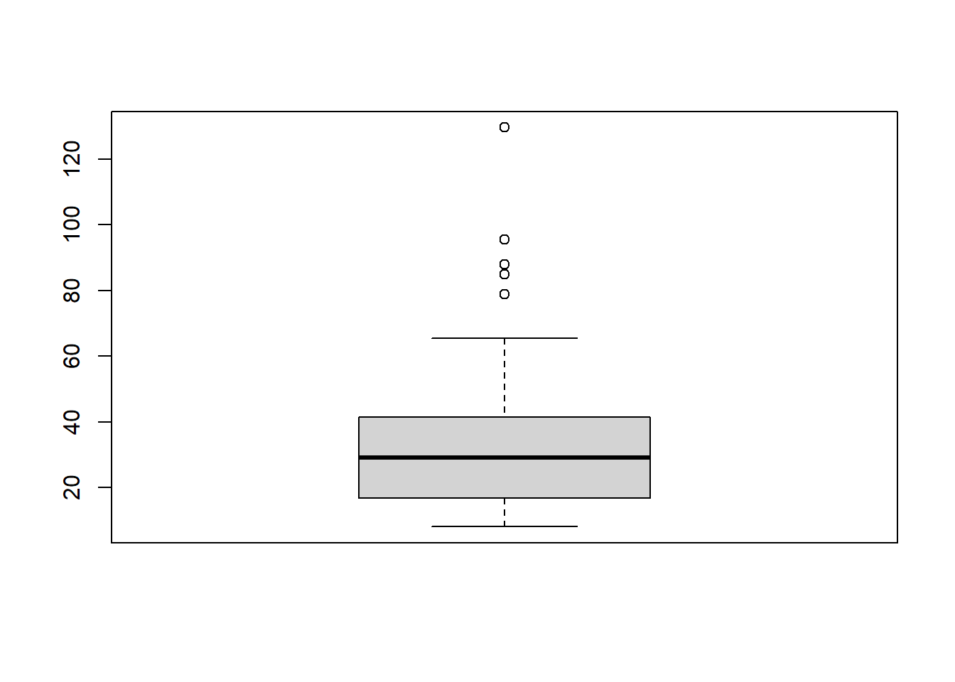
Provide descriptive statistics for each variable in the dataset.

Solution

We now inspect some descriptive statistics for each variable in the dataset:

# Quick summary
summary(job)

     commun       probl_solv      logical       learn         physical   
 Min.   :12.0   Min.   :48.0   Min.   :20   Min.   :44.0   Min.   :48.0  
 1st Qu.:16.0   1st Qu.:52.2   1st Qu.:22   1st Qu.:48.0   1st Qu.:52.2  
 Median :18.0   Median :54.0   Median :24   Median :50.0   Median :54.0  
 Mean   :17.7   Mean   :54.2   Mean   :24   Mean   :50.3   Mean   :54.2  
 3rd Qu.:19.8   3rd Qu.:56.0   3rd Qu.:26   3rd Qu.:52.0   3rd Qu.:56.0  
 Max.   :24.0   Max.   :59.0   Max.   :31   Max.   :56.0   Max.   :59.0  
   appearance    arrest_rate   
 Min.   :16.0   Min.   :0.000  
 1st Qu.:19.0   1st Qu.:0.371  
 Median :21.0   Median :0.565  
 Mean   :21.1   Mean   :0.512  
 3rd Qu.:23.0   3rd Qu.:0.669  
 Max.   :28.0   Max.   :0.935  

OPTIONAL

If you wish to create a nice looking table for a report, you could try the following code. However, I should warn you: this code is quite difficult to understand so, if you are interested, attend a lab!

library(gt)

# Mean and SD of each variable
job %>% 
  summarise(across(everything(), list(M = mean, SD = sd))) %>%
  pivot_longer(everything()) %>% 
  mutate(
    value = round(value, 2),
    name = str_replace(name, '_M', '.M'),
    name = str_replace(name, '_SD', '.SD')
  ) %>%
  separate(name, into = c('variable', 'summary'), sep = '\\.') %>%
  pivot_wider(names_from = summary, values_from = value) %>% 
  gt()

variable	M	SD
commun	17.68	2.74
probl_solv	54.16	2.41
logical	24.02	2.49
learn	50.28	2.84
physical	54.16	2.41
appearance	21.06	2.99
arrest_rate	0.51	0.23

2. Is PCA needed?

There are many reasons we might want to reduce the dimensionality of data:

• Theory testing
  • What are the number and nature of dimensions that best describe a theoretical construct?
• Test construction
  • How should I group my items into sub-scales?
  • Which items are the best measures of my constructs?
• Pragmatic
  • I have multicollinearity issues/too many variables, how can I defensibly combine my variables?

PCA is most often used for the latter - we are less interested in the theory behind our items, we just want a useful way of simplifying lots of variables down to a smaller number.

Recall that we are wanting to see how well the skills ratings predict arrest rate.
We might fit this model:

mod <- lm(arrest_rate ~ commun + probl_solv + logical + learn + physical + appearance, data = job)

However, we might have reason to think that many of these predictors might be quite highly correlated with one another, and so we may be unable to draw accurate inferences. This is borne out in our variance inflation factor (VIF):

library(car)
vif(mod)

    commun probl_solv    logical      learn   physical appearance 
     34.67       1.17       1.23      43.56      34.98      21.78 

As the original variables are highly correlated, it is possible to reduce the dimensionality of the problem under investigation without losing too much information.

On the other side, if the correlation between the variables under study are weak, a larger number of components is needed in order to explain sufficient variability.

Question A3

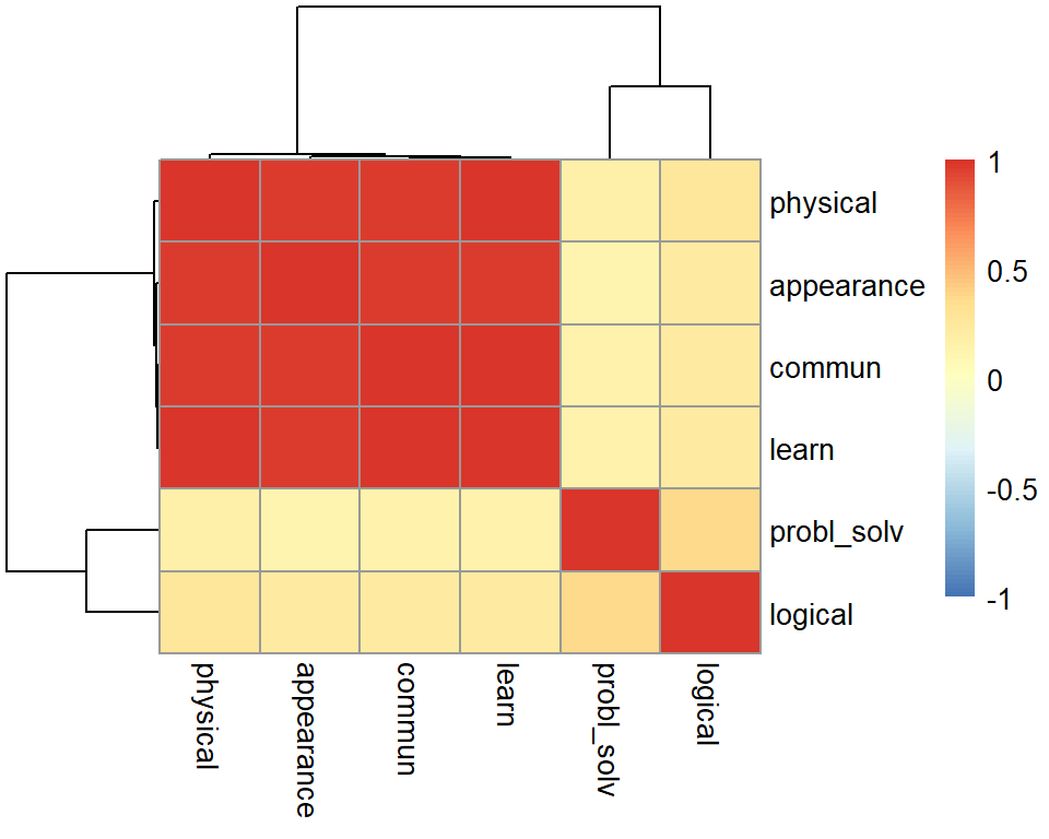
Working with only the skills ratings (not the arrest rate - we’ll come back to that right at the end), investigate whether or not the variables are highly correlated and explain whether or not you PCA might be useful in this case.

Hint: We only have 6 variables here, but if we had many, how might you visualise cor(job)?

Solution

Let’s start by looking at the correlation matrix of the data:

library(pheatmap)

job_skills <- job %>% select(-arrest_rate)

R <- cor(job_skills)

pheatmap(R, breaks = seq(-1, 1, length.out = 100))

Figure 1: Correlation between the variables in the ``Job’’ dataset

The correlation between the variables seems to be quite large (it doesn’t matter about direction here, only magnitude; if negative correlations were present, we would think in absolute value).

There appears to be a group of highly correlated variables comprising physical ability, appearance, communication skills, and learning ability which are correlated among themselves but uncorrelated with another group of variables. The second group comprises problem solving and logical ability.

This suggests that PCA might be useful in this problem to reduce the dimensionality without a significant loss of information.

3. Cov vs Cor?

Should we perform PCA on the covariance or the correlation matrix?

This depends on the variances of the variables in the dataset. If the variables have large differences in their variances, then the variables with the largest variances will tend to dominate the first few principal components.
A solution to this is to standardise the variables prior to computing the covariance matrix - i.e., compute the correlation matrix!

# show that the correlation matrix and the covariance matrix of the standardized variables are identical
all.equal(cor(job_skills), cov(scale(job_skills)))

[1] TRUE

Question A4

Look at the variance of the skills ratings in the data set. Do you think that PCA should be carried on the covariance matrix or the correlation matrix?

Solution

Let’s have a look at the standard deviation of each variable:

job_skills %>% 
  summarise(across(everything(), sd))

# A tibble: 1 × 6
  commun probl_solv logical learn physical appearance
   <dbl>      <dbl>   <dbl> <dbl>    <dbl>      <dbl>
1   2.74       2.41    2.49  2.84     2.41       2.99

As the standard deviations appear to be fairly similar (and so will the variances) we can perform PCA using the covariance matrix.

4. Perform PCA

Question A5

Using the principal() function from the psych package, we can perform a PCA of the job performance data, Call the output job_pca.

job_pca <- principal(job_skills, nfactors = ncol(job_skills), covar = ..., rotate = 'none')
job_pca$loadings

Depending on your answer to the previous question, either set covar = TRUE or covar = FALSE within the principal() function.

Warning: the output of the function will be in terms of standardized variables nevertheless. So you will see output with standard deviation of 1.

Solution

library(psych)

job_pca <- principal(job_skills, nfactors = ncol(job_skills), covar = TRUE, rotate = 'none')

PCA OUTPUT

We can print the output by just typing the name of our PCA:

job_pca

Principal Components Analysis
Call: principal(r = job_skills, nfactors = ncol(job_skills), rotate = "none", 
    covar = TRUE)
Standardized loadings (pattern matrix) based upon correlation matrix
            PC1   PC2   PC3   PC4   PC5   PC6 h2       u2 com
commun     0.98 -0.12  0.02 -0.06  0.10 -0.05  1  6.7e-16 1.1
probl_solv 0.22  0.81  0.54  0.00  0.00  0.00  1  1.1e-15 1.9
logical    0.33  0.75 -0.58  0.00  0.00  0.00  1  1.1e-15 2.3
learn      0.99 -0.11  0.02 -0.05  0.00  0.11  1  0.0e+00 1.1
physical   0.99 -0.08  0.01 -0.05 -0.11 -0.05  1 -4.4e-16 1.0
appearance 0.98 -0.13  0.02  0.16  0.01  0.00  1  2.2e-16 1.1

                       PC1  PC2  PC3  PC4  PC5  PC6
SS loadings           4.04 1.26 0.63 0.03 0.02 0.02
Proportion Var        0.67 0.21 0.11 0.01 0.00 0.00
Cumulative Var        0.67 0.88 0.99 0.99 1.00 1.00
Proportion Explained  0.67 0.21 0.11 0.01 0.00 0.00
Cumulative Proportion 0.67 0.88 0.99 0.99 1.00 1.00

Mean item complexity =  1.4
Test of the hypothesis that 6 components are sufficient.

The root mean square of the residuals (RMSR) is  0 
 with the empirical chi square  0  with prob <  NA 

Fit based upon off diagonal values = 1

The output is made up of two parts.

First, it shows the loading matrix. In each column of the loading matrix we find how much each of the measured variables contributes to the computed new axis/direction (that is, the principal component). Notice that there are as many principal components as variables.

The second part of the output displays the contribution of each component to the total variance:

• SS loadings: The sum of the squared loadings. The eigenvalues (see Lecture).
  
• Proportion Var: how much of the overall variance the component accounts for out of all the variables.
• Cumulative Var: cumulative sum of Proportion Var.
• Proportion Explained: relative amount of variance explained (\(\frac{\text{Proportion Var}}{\text{sum(Proportion Var)}}\).
• Cumulative Proportion: cumulative sum of Proportion Explained.

Let’s focus on the row of that output called “Cumulative Var”. This displays the cumulative sum of the variances of each principal component. Taken all together, the six principal components taken explain all of the total variance in the original data. In other words, the total variance of the principal components (the sum of their variances) is equal to the total variance in the original data (the sum of the variances of the variables).

However, our goal is to reduce the dimensionality of our data, so it comes natural to wonder which of the six principal components explain most of the variability, and which components instead do not contribute substantially to the total variance.

To that end, the second row “Proportion Var” displays the proportion of the total variance explained by each component, i.e. the variance of the principal component divided by the total variance.

The last row, as we saw, is the cumulative proportion of explained variance: 0.67, 0.67 + 0.21, 0.67 + 0.21 + 0.11, and so on.

We also notice that the first PC alone explains 67.3% of the total variability, while the first two components together explain almost 90% of the total variability. From the third component onwards, we do not see such a sharp increase in the proportion of explained variance, and the cumulative proportion slowly reaches the total ratio of 1 (or 100%).

Optional: (some of) the math behind it

Doing data reduction can feel a bit like magic, and in part that’s just because it’s quite complicated.

The intuition

Consider one way we might construct a correlation matrix - as the product of vector \(\mathbf{f}\) with \(\mathbf{f'}\) (f transposed):

\[ \begin{equation*} \mathbf{f} = \begin{bmatrix} 0.9 \\ 0.8 \\ 0.7 \\ 0.6 \\ 0.5 \\ 0.4 \\ \end{bmatrix} \qquad \mathbf{f} \mathbf{f'} = \begin{bmatrix} 0.9 \\ 0.8 \\ 0.7 \\ 0.6 \\ 0.5 \\ 0.4 \\ \end{bmatrix} \begin{bmatrix} 0.9, 0.8, 0.7, 0.6, 0.5, 0.4 \\ \end{bmatrix} \qquad = \qquad \begin{bmatrix} 0.81, 0.72, 0.63, 0.54, 0.45, 0.36 \\ 0.72, 0.64, 0.56, 0.48, 0.40, 0.32 \\ 0.63, 0.56, 0.49, 0.42, 0.35, 0.28 \\ 0.54, 0.48, 0.42, 0.36, 0.30, 0.24 \\ 0.45, 0.40, 0.35, 0.30, 0.25, 0.20 \\ 0.36, 0.32, 0.28, 0.24, 0.20, 0.16 \\ \end{bmatrix} \end{equation*} \]

But we constrain this such that the diagonal has values of 1 (the correlation of a variable with itself is 1), and lets call it R.

\[ \begin{equation*} \mathbf{R} = \begin{bmatrix} 1.00, 0.72, 0.63, 0.54, 0.45, 0.36 \\ 0.72, 1.00, 0.56, 0.48, 0.40, 0.32 \\ 0.63, 0.56, 1.00, 0.42, 0.35, 0.28 \\ 0.54, 0.48, 0.42, 1.00, 0.30, 0.24 \\ 0.45, 0.40, 0.35, 0.30, 1.00, 0.20 \\ 0.36, 0.32, 0.28, 0.24, 0.20, 1.00 \\ \end{bmatrix} \end{equation*} \]

PCA is about trying to determine a vector f which generates the correlation matrix R. a bit like unscrambling eggs!

in PCA, we express \(\mathbf{R = CC'}\), where \(\mathbf{C}\) are our principal components.
If \(n\) is number of variables in \(R\), then \(i^{th}\) component \(C_i\) is the linear sum of each variable multiplied by some weighting:

\[ C_i = \sum_{j=1}^{n}w_{ij}x_{j} \]

How do we find \(C\)?

This is where “eigen decomposition” comes in.
For the \(n \times n\) correlation matrix \(\mathbf{R}\), there is an eigenvector \(x_i\) that solves the equation

\[ \mathbf{x_i R} = \lambda_i \mathbf{x_i} \]

Where the vector multiplied by the correlation matrix is equal to some eigenvalue \(\lambda_i\) multiplied by that vector.
We can write this without subscript \(i\) as:

\[ \begin{align} & \mathbf{R X} = \mathbf{X \lambda} \\ & \text{where:} \\ & \mathbf{R} = \text{correlation matrix} \\ & \mathbf{X} = \text{matrix of eigenvectors} \\ & \mathbf{\lambda} = \text{vector of eigenvalues} \end{align} \]

the vectors which make up \(\mathbf{X}\) must be orthogonal (\(\mathbf{XX' = I}\)), which means that \(\mathbf{R = X \lambda X'}\)

We can actually do this in R manually. Creating a correlation matrix

# lets create a correlation matrix, as the produce of ff'
f <- seq(.9,.4,-.1)
R <- f %*% t(f)
#give rownames and colnames
rownames(R)<-colnames(R)<-paste0("V",seq(1:6))
#constrain diagonals to equal 1
diag(R)<-1
R

     V1   V2   V3   V4   V5   V6
V1 1.00 0.72 0.63 0.54 0.45 0.36
V2 0.72 1.00 0.56 0.48 0.40 0.32
V3 0.63 0.56 1.00 0.42 0.35 0.28
V4 0.54 0.48 0.42 1.00 0.30 0.24
V5 0.45 0.40 0.35 0.30 1.00 0.20
V6 0.36 0.32 0.28 0.24 0.20 1.00

Eigen Decomposition

# do eigen decomposition
e <- eigen(R)
print(e, digits=2)

eigen() decomposition
$values
[1] 3.16 0.82 0.72 0.59 0.44 0.26

$vectors
      [,1]   [,2]   [,3]  [,4]   [,5]   [,6]
[1,] -0.50 -0.061  0.092  0.14  0.238  0.816
[2,] -0.47 -0.074  0.121  0.21  0.657 -0.533
[3,] -0.43 -0.096  0.182  0.53 -0.675 -0.184
[4,] -0.39 -0.142  0.414 -0.78 -0.201 -0.104
[5,] -0.34 -0.299 -0.860 -0.20 -0.108 -0.067
[6,] -0.28  0.934 -0.178 -0.10 -0.067 -0.045

The eigenvectors are orthogonal (\(\mathbf{XX' = I}\)):

round(e$vectors %*% t(e$vectors),2)

     [,1] [,2] [,3] [,4] [,5] [,6]
[1,]    1    0    0    0    0    0
[2,]    0    1    0    0    0    0
[3,]    0    0    1    0    0    0
[4,]    0    0    0    1    0    0
[5,]    0    0    0    0    1    0
[6,]    0    0    0    0    0    1

The Principal Components \(\mathbf{C}\) are the eigenvectors scaled by the square root of the eigenvalues:

#eigenvectors
e$vectors

       [,1]    [,2]    [,3]   [,4]    [,5]    [,6]
[1,] -0.496 -0.0611  0.0923  0.139  0.2385  0.8155
[2,] -0.468 -0.0743  0.1210  0.214  0.6566 -0.5327
[3,] -0.433 -0.0963  0.1820  0.530 -0.6751 -0.1842
[4,] -0.390 -0.1416  0.4143 -0.778 -0.2006 -0.1036
[5,] -0.340 -0.2992 -0.8604 -0.197 -0.1076 -0.0669
[6,] -0.282  0.9338 -0.1784 -0.100 -0.0667 -0.0452

#scaled by sqrt of eigenvalues
diag(sqrt(e$values))

     [,1]  [,2]  [,3]  [,4]  [,5]  [,6]
[1,] 1.78 0.000 0.000 0.000 0.000 0.000
[2,] 0.00 0.906 0.000 0.000 0.000 0.000
[3,] 0.00 0.000 0.848 0.000 0.000 0.000
[4,] 0.00 0.000 0.000 0.769 0.000 0.000
[5,] 0.00 0.000 0.000 0.000 0.664 0.000
[6,] 0.00 0.000 0.000 0.000 0.000 0.512

C <- e$vectors %*% diag(sqrt(e$values))
C

       [,1]    [,2]    [,3]    [,4]    [,5]    [,6]
[1,] -0.883 -0.0554  0.0782  0.1070  0.1584  0.4174
[2,] -0.833 -0.0673  0.1025  0.1648  0.4361 -0.2727
[3,] -0.770 -0.0873  0.1542  0.4077 -0.4483 -0.0943
[4,] -0.694 -0.1284  0.3512 -0.5987 -0.1332 -0.0530
[5,] -0.604 -0.2712 -0.7293 -0.1514 -0.0715 -0.0342
[6,] -0.502  0.8464 -0.1513 -0.0771 -0.0443 -0.0231

And we can reproduce our correlation matrix, because \(\mathbf{R = CC'}\).

C %*% t(C)

     [,1] [,2] [,3] [,4] [,5] [,6]
[1,] 1.00 0.72 0.63 0.54 0.45 0.36
[2,] 0.72 1.00 0.56 0.48 0.40 0.32
[3,] 0.63 0.56 1.00 0.42 0.35 0.28
[4,] 0.54 0.48 0.42 1.00 0.30 0.24
[5,] 0.45 0.40 0.35 0.30 1.00 0.20
[6,] 0.36 0.32 0.28 0.24 0.20 1.00

Now lets imagine we only consider 1 principal component.
We can do this with the principal() function:

library(psych)
pc1<-principal(R, nfactors = 1, covar = FALSE, rotate = 'none')
pc1

Principal Components Analysis
Call: principal(r = R, nfactors = 1, rotate = "none", covar = FALSE)
Standardized loadings (pattern matrix) based upon correlation matrix
    PC1   h2   u2 com
V1 0.88 0.78 0.22   1
V2 0.83 0.69 0.31   1
V3 0.77 0.59 0.41   1
V4 0.69 0.48 0.52   1
V5 0.60 0.37 0.63   1
V6 0.50 0.25 0.75   1

                PC1
SS loadings    3.16
Proportion Var 0.53

Mean item complexity =  1
Test of the hypothesis that 1 component is sufficient.

The root mean square of the residuals (RMSR) is  0.09 

Fit based upon off diagonal values = 0.95

Look familiar? It looks like the first component we computed manually. The first column of \(\mathbf{C}\):

cbind(pc1$loadings, C=C[,1])

     PC1      C
V1 0.883 -0.883
V2 0.833 -0.833
V3 0.770 -0.770
V4 0.694 -0.694
V5 0.604 -0.604
V6 0.502 -0.502

We can now ask “how well does this component (on its own) recreate our correlation matrix?”

C[,1] %*% t(C[,1])

      [,1]  [,2]  [,3]  [,4]  [,5]  [,6]
[1,] 0.780 0.735 0.680 0.613 0.534 0.444
[2,] 0.735 0.693 0.641 0.578 0.503 0.418
[3,] 0.680 0.641 0.592 0.534 0.465 0.387
[4,] 0.613 0.578 0.534 0.481 0.419 0.348
[5,] 0.534 0.503 0.465 0.419 0.365 0.304
[6,] 0.444 0.418 0.387 0.348 0.304 0.252

It looks close, but not quite. How much not quite? Measurably so!

R - (C[,1] %*% t(C[,1]))

        V1      V2      V3      V4      V5      V6
V1  0.2200 -0.0154 -0.0498 -0.0727 -0.0838 -0.0836
V2 -0.0154  0.3067 -0.0809 -0.0976 -0.1033 -0.0982
V3 -0.0498 -0.0809  0.4075 -0.1140 -0.1153 -0.1066
V4 -0.0727 -0.0976 -0.1140  0.5187 -0.1193 -0.1085
V5 -0.0838 -0.1033 -0.1153 -0.1193  0.6346 -0.1036
V6 -0.0836 -0.0982 -0.1066 -0.1085 -0.1036  0.7477

Notice the values on the diagonals of \(\mathbf{c_1}\mathbf{c_1}'\).

diag(C[,1] %*% t(C[,1]))

[1] 0.780 0.693 0.592 0.481 0.365 0.252

These aren’t 1, like they are in \(R\). But they are proportional: this is the amount of variance in each observed variable that is explained by this first component. Sound familiar?

pc1$communality

   V1    V2    V3    V4    V5    V6 
0.780 0.693 0.592 0.481 0.365 0.252 

And likewise the 1 minus these is the unexplained variance:

1 - diag(C[,1] %*% t(C[,1]))

[1] 0.220 0.307 0.408 0.519 0.635 0.748

pc1$uniquenesses

   V1    V2    V3    V4    V5    V6 
0.220 0.307 0.408 0.519 0.635 0.748 

5. How many components to keep?

There is no single best method to select the optimal number of components to keep, while discarding the remaining ones (which are then considered as noise components).

The following three heuristic rules are commonly used in the literature:

• The cumulative proportion of explained variance criterion
• Kaiser’s rule
• The scree plot
• Velicer’s Minimum Average Partial method
• Parallel analysis

In the next sections we will analyse each of them in turn.

The cumulative proportion of explained variance criterion

The rule suggests to keep as many principal components as needed in order to explain approximately 80-90% of the total variance.

Question A6

Looking again at the PCA output, how many principal components would you keep if you were following the cumulative proportion of explained variance criterion?

Solution

Let’s look again at the PCA summary:

job_pca$loadings

Loadings:
           PC1    PC2    PC3    PC4    PC5    PC6   
commun      0.984 -0.120                0.101       
probl_solv  0.223  0.810  0.543                     
logical     0.329  0.747 -0.578                     
learn       0.987 -0.110                       0.105
physical    0.988                      -0.110       
appearance  0.979 -0.125         0.161              

                 PC1   PC2   PC3   PC4   PC5   PC6
SS loadings    4.035 1.261 0.631 0.035 0.022 0.016
Proportion Var 0.673 0.210 0.105 0.006 0.004 0.003
Cumulative Var 0.673 0.883 0.988 0.994 0.997 1.000

The following part of the output tells us that the first two components explain 88.3% of the total variance.

Cumulative Var 0.673 0.883 0.988 0.994 0.997 1.000

According to this criterion, we should keep 2 principal components.

Kaiser’s rule

According to Kaiser’s rule, we should keep the principal components having variance larger than 1. Standardized variables have a variance equal 1. Because we have 6 variables in the data set, and the total variance is 6, the value 1 represents the average variance in the data:

\[ \frac{1 + 1 + 1 + 1 + 1 + 1}{6} = 1 \]

Hint:

The variances of each PC are shown in the row of the output named SS loadings and also in job_pca$values. The average variance is:

mean(job_pca$values)

[1] 1

Question A7

Looking again at the PCA output, how many principal components would you keep if you were following Kaiser’s criterion?

Solution

job_pca$loadings

Loadings:
           PC1    PC2    PC3    PC4    PC5    PC6   
commun      0.984 -0.120                0.101       
probl_solv  0.223  0.810  0.543                     
logical     0.329  0.747 -0.578                     
learn       0.987 -0.110                       0.105
physical    0.988                      -0.110       
appearance  0.979 -0.125         0.161              

                 PC1   PC2   PC3   PC4   PC5   PC6
SS loadings    4.035 1.261 0.631 0.035 0.022 0.016
Proportion Var 0.673 0.210 0.105 0.006 0.004 0.003
Cumulative Var 0.673 0.883 0.988 0.994 0.997 1.000

The variances are shown in the row

SS loadings    4.035 1.261 0.631 0.035 0.022 0.016

From the result we see that only the first two principal components have variance greater than 1, so this rule suggests to keep 2 PCs only.

The scree plot

The scree plot is a graphical criterion which involves plotting the variance for each principal component. This can be easily done by calling plot on the variances, which are stored in job_pca$values

plot(x = 1:length(job_pca$values), y = job_pca$values, 
     type = 'b', xlab = '', ylab = 'Variance', 
     main = 'Police officers: scree plot', frame.plot = FALSE)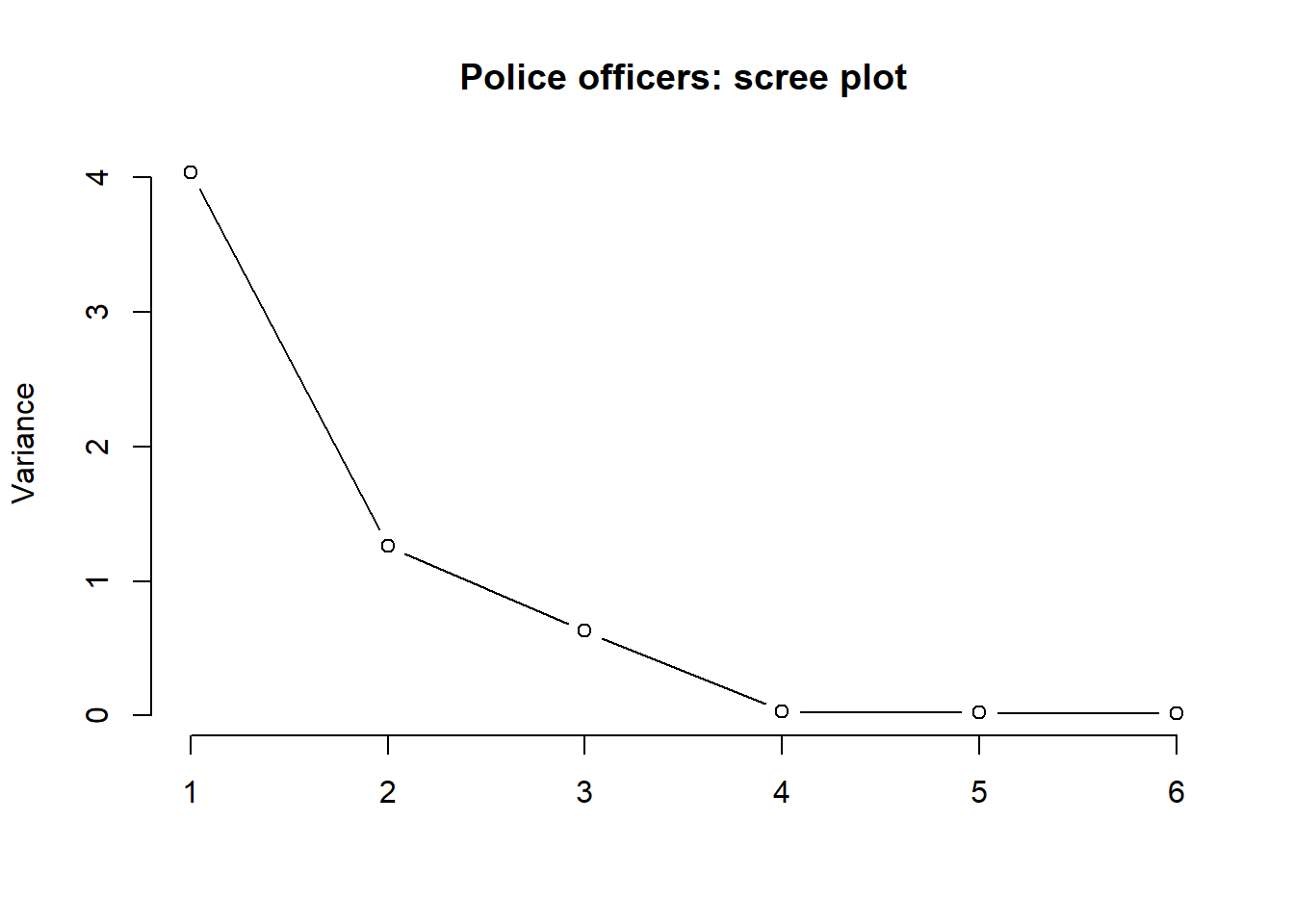

where the argument type = 'b' tells R that the plot should have both points and lines.

A typical scree plot features higher variances for the initial components and quickly drops to small variances where the curve is almost flat. The flat part of the curve represents the noise components, which are not able to capture the main sources of variability in the system.

According to the scree plot criterion, we should keep as many principal components as where the “elbow” in the plot occurs. By elbow we mean the variance before the curve looks almost flat.

Alternatively, some people prefer to use the function scree() from the psych package:

scree(job_skills, factors = FALSE)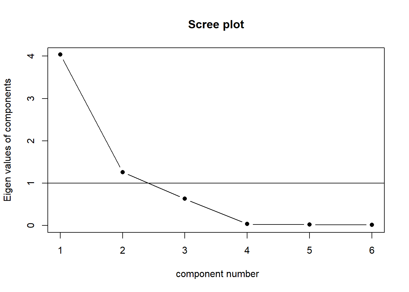

This also draws a horizontal line at y = 1. So, if you are making a decision about how many PCs to keep by looking at where the plot falls below the y = 1 line, you are basically following Kaiser’s rule. In fact, Kaiser’s criterion tells you to keep as many PCs as are those with a variance (= eigenvalue) greater than 1.

Question A8

According to the scree plot, how many principal components would you retain?

Solution

This criterion then suggests to keep three principal components.

Velicer’s Minimum Average Partial method

The Minimum Average Partial (MAP) test computes the partial correlation matrix (removing and adjusting for a component from the correlation matrix), sequentially partialling out each component. At each step, the partial correlations are squared and their average is computed.
At first, the components which are removed will be those that are most representative of the shared variance between 2+ variables, meaning that the “average squared partial correlation” will decrease. At some point in the process, the components being removed will begin represent variance that is specific to individual variables, meaning that the average squared partial correlation will increase.
The MAP method is to keep the number of components for which the average squared partial correlation is at the minimum.

We can conduct MAP in R using:

VSS(data, plot = FALSE, method="pc", n = ncol(data))

(be aware there is a lot of other information in this output too! For now just focus on the map column)

Question A9

How many components should we keep according to the MAP method?

Solution

job_map <- VSS(job_skills, plot=FALSE, method="pc", n = ncol(job_skills))$map
paste("MAP is lowest for", which.min(job_map), "components")

[1] "MAP is lowest for 2 components"

According to the MAP criterion we should keep 2 principal components.

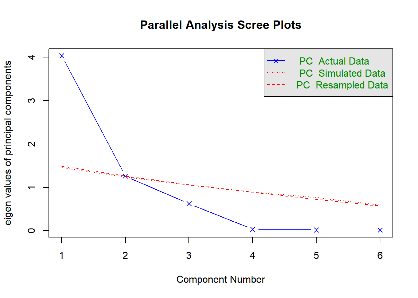
Parallel analysis

Parallel analysis involves simulating lots of datasets of the same dimension but in which the variables are uncorrelated. For each of these simulations, a PCA is conducted on its correlation matrix, and the eigenvalues are extracted. We can then compare our eigenvalues from the PCA on our actual data to the average eigenvalues across these simulations. In theory, for uncorrelated variables, no components should explain more variance than any others, and eigenvalues should be equal to 1. In reality, variables are rarely truly uncorrelated, and so there will be slight variation in the magnitude of eigenvalues simply due to chance. The parallel analysis method suggests keeping those components for which the eigenvalues are greater than those from the simulations.

It can be conducted in R using:

fa.parallel(job_skills, fa="pc", quant=.95)

Question A10

How many components should we keep according to parallel analysis?

Solution

fa.parallel(job_skills, fa="pc", quant=.95)

Parallel analysis suggests that the number of factors =  NA  and the number of components =  1 

Parallel analysis suggests to keep 1 principal component only as there is only one PC with an eigenvalue higher than the simulated random ones in red.

Interpretation

Because three out of the five selection criteria introduced above suggest to keep 2 principal components, in the following we will work with the first two PCs only.

Let’s have a look at the selected principal components:

job_pca$loadings[, 1:2]

             PC1     PC2
commun     0.984 -0.1197
probl_solv 0.223  0.8095
logical    0.329  0.7466
learn      0.987 -0.1097
physical   0.988 -0.0784
appearance 0.979 -0.1253

and at their corresponding proportion of total variance explained:

job_pca$values / sum(job_pca$values)

[1] 0.67253 0.21016 0.10510 0.00577 0.00372 0.00273

We see that the first PC accounts for 67.3% of the total variability. All loadings seem to have the same magnitude apart from probl_solv and logical which are closer to zero. The first component looks like a sort of average of the officers performance scores excluding problem solving and logical ability.

The second principal component, which explains only 21% of the total variance, has two loadings clearly distant from zero: the ones associated to problem solving and logical ability. It distinguishes police officers with strong logical and problem solving skills and low scores on other skills (note the negative magnitudes).

We have just seen how to interpret the first components by looking at the magnitude and sign of the coefficients for each measured variable.

For interpretation purposes, it might help hiding very small loadings. This can be done by specifying the cutoff value in the print() function. However, this only works when you pass the loadings for all the PCs:

print(job_pca$loadings, cutoff = 0.3)

Loadings:
           PC1    PC2    PC3    PC4    PC5    PC6   
commun      0.984                                   
probl_solv         0.810  0.543                     
logical     0.329  0.747 -0.578                     
learn       0.987                                   
physical    0.988                                   
appearance  0.979                                   

                 PC1   PC2   PC3   PC4   PC5   PC6
SS loadings    4.035 1.261 0.631 0.035 0.022 0.016
Proportion Var 0.673 0.210 0.105 0.006 0.004 0.003
Cumulative Var 0.673 0.883 0.988 0.994 0.997 1.000

Optional: How well are the units represented in the reduced space?

We now focus our attention on the following question: Are all the statistical units (police officers) well represented in the 2D plot?

The 2D representation of the original data, which comprise 6 measured variables, is an approximation and henceforth it may happen that not all units are well represented in this new space.

Typically, it is good to assess the approximation for each statistical unit by inspecting the scores on the discarded principal components. If a unit has a high score on those components, then this is a sign that the unit might be highly misplaced in the new space and misrepresented.

Consider the 3D example below. There are three cases (= units or individuals). In the original space they are all very different from each other. For example, cases 1 and 2 are very different in their x and y values, but very similar in their z value. Cases 2 and 3 are very similar in their x and y values but very different in their z value. Cases 1 and 3 have very different values for all three variables x, y, and z.

However, when represented in the 2D space given by the two principal components, units 2 and 3 seems like they are very similar when, in fact, they were very different in the original space which also accounted for the z variable.

We typically measure how badly a unit is represented in the new coordinate system by considering the sum of squared scores on the discarded principal components:

scores_discarded <- job_pca$scores[, -(1:2)]
sum_sq <- rowSums(scores_discarded^2)
sum_sq

 [1]  28.51  46.89  63.69  64.24  36.58  17.39  49.24  35.10  18.56  19.27
[11]  18.56  24.44  12.39  59.10  24.43  33.18  13.40  12.69  11.22  78.87
[21]  14.16  34.18  95.57  18.40  16.45  14.41  31.97  33.52  40.12  32.48
[31]  16.85  24.85  30.84  16.00  29.59  11.01   8.07  18.18  14.60  23.73
[41]  29.82  41.37   9.30  65.42  21.98  63.97  36.09  84.98 129.65  88.00

Units with a high score should be considered for further inspection as it may happen that they are represented as close to another unit when, in fact, they might be very different.

boxplot(sum_sq)

There seem to be only five outliers, and they are not too high compared to the rest of the scores. For this reason, we will consider the 2D representation of the data to be satisfactory.

6. Using PCA scores

Supposing that we decide to reduce our six variables down to two principal components:

job_pca2 <- principal(job_skills, nfactors = 2, covar = TRUE, rotate = 'none')

We can, for each of our observations, get their scores on each of our components.

head(job_pca2$scores)

       PC1    PC2
[1,] -6.10 -1.796
[2,] -4.69  4.164
[3,] -5.18 -0.131
[4,] -4.31 -1.758
[5,] -3.71  1.207
[6,] -3.88 -5.200

In the literature, some authors also suggest to look at the correlation between each principal component and the measured variables:

# First PC
cor(job_pca2$scores[,1], job_skills)

     commun probl_solv logical learn physical appearance
[1,]  0.985      0.214   0.319 0.988    0.989      0.981

The first PC is strongly correlated with all the measured variables except probl_solv and logical. As we mentioned above, all variables seem to contributed to the first PC.

# Second PC
cor(job_pca2$scores[,2], job_skills)

     commun probl_solv logical  learn physical appearance
[1,] -0.163      0.792   0.738 -0.154   -0.122     -0.169

The second PC is strongly correlated with probl_solv and logical, and slightly negatively correlated with the remaining variables. This separates police officers with clear logical and problem solving skills and a low rating on other skills.

Question A11

We have reduced our six variables down to two principal components, and we are now able to use the scores on each component in a subsequent analysis!

Join the two PC scores to the original dataset with the arrest rates in. Then fit a linear model to look at how the arrest rate of police officers is predicted by the two components representing different composites of the skills ratings by HR.

Solution

# add the PCA scores to the dataset
job <- 
  job %>% mutate(
    pc1 = job_pca2$scores[,1],
    pc2 = job_pca2$scores[,2]
  )
# use the scores in an analysis
mod <- lm(arrest_rate ~ pc1 + pc2, data = job)

# multicollinearity isn't a problem, because the components are orthogonal!! 
library(car)
vif(mod)

pc1 pc2 
  1   1 

summary(mod)

Call:
lm(formula = arrest_rate ~ pc1 + pc2, data = job)

Residuals:
   Min     1Q Median     3Q    Max 
-0.385 -0.119 -0.016  0.160  0.384 

Coefficients:
            Estimate Std. Error t value Pr(>|t|)    
(Intercept)  0.51161    0.02943   17.38   <2e-16 ***
pc1          0.03583    0.01089    3.29   0.0019 ** 
pc2         -0.00923    0.01210   -0.76   0.4490    
---
Signif. codes:  0 '***' 0.001 '**' 0.01 '*' 0.05 '.' 0.1 ' ' 1

Residual standard error: 0.208 on 47 degrees of freedom
Multiple R-squared:   0.2,  Adjusted R-squared:  0.166 
F-statistic: 5.86 on 2 and 47 DF,  p-value: 0.00532

Plotting PCA scores

We can also visualise the statistical units (police officers) in the reduced space given by the retained principal component scores.

tibble(pc1 = job_pca2$scores[, 1],
       pc2 = job_pca2$scores[, 2]) %>%
  ggplot(.,aes(x=pc1,y=pc2))+
  geom_point()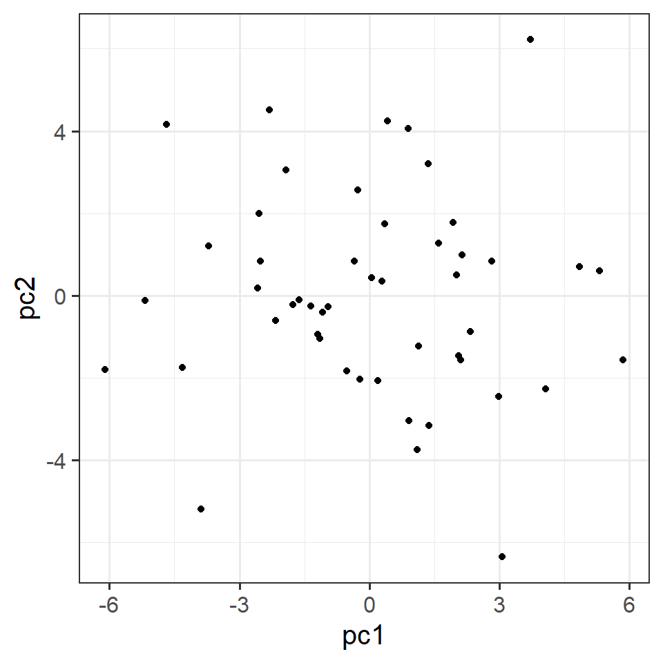

Footnotes

1. Even if we cut open someone’s brain, it’s unclear what we would be looking for in order to ‘measure’ it. It is unclear whether anxiety even exists as a physical thing, or rather if it is simply the overarching concept we apply to a set of behaviours and feelings