Exploratory Factor Analysis (EFA): Part 1

Relevant packages

• psych
• GPArotation

PCA vs FA

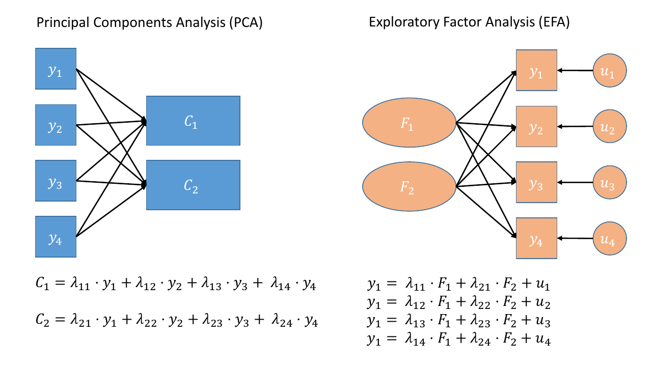
Where PCA aims to summarise a set of measured variables into a set of orthogonal (uncorrelated) components as linear combinations (a weighted average) of the measured variables, Factor Analysis (FA) assumes that the relationships between a set of measured variables can be explained by a number of underlying latent factors.

Note how the directions of the arrows in Figure 1 are different between PCA and FA - in PCA, each component \(C_i\) is the weighted combination of the observed variables \(y_1, ...,y_n\), whereas in FA, each measured variable \(y_i\) is seen as generated by some latent factor(s) \(F_i\) plus some unexplained variance \(u_i\).

It might help to read the \(\lambda\)s as beta-weights (\(b\), or \(\beta\)), because that’s all they really are. The equation \(y_i = \lambda_{1i} F_1 + \lambda_{2i} F_2 + u_i\) is just our way of saying that the variable \(y_i\) is the manifestation of some amount (\(\lambda_{1i}\)) of an underlying factor \(F_1\), some amount (\(\lambda_{2i}\)) of some other underlying factor \(F_2\), and some error (\(u_i\)).

Figure 1: Path diagrams for PCA and FA

In Exploratory Factor Analysis (EFA), we are starting with no hypothesis about either the number of latent factors or about the specific relationships between latent factors and measured variables (known as the factor structure). Typically, all variables will load on all factors, and a transformation method such as a rotation (we’ll cover this in more detail below) is used to help make the results more easily interpretable.¹

Suitability of items for EFA

There are various ways of assessing the suitability of our items for exploratory factor analysis, and most of them rely on examining the observed correlations between items.

Look at the correlation matrix

Use a function such as cor or corr.test(data) (from the psych package) to create the correlation matrix.

Bartlett’s Test

The function cortest.bartlett(cor(data), n = nrow(data)) conducts “Bartlett’s test”. This tests against the null that the correlation matrix is proportional to the identity matrix (a matrix of all 0s except for 1s on the diagonal).

• Null hypothesis: observed correlation matrix is equivalent to the identity matrix
  
• Alternative hypothesis: observed correlation matrix is not equivalent to the identity matrix.

What is the identity matrix?

The “Identity matrix” is a matrix of all 0s except for 1s on the diagonal.
e.g. for a 3x3 matrix:

\[ \begin{bmatrix} 1 & 0 & 0 \\ 0 & 1 & 0 \\ 0 & 0 & 1 \\ \end{bmatrix} \]

If a correlation matrix looks like this, then it means there is no shared variance between the items, so it is not suitable for factor analysis

Kaiser, Meyer, Olkin Measure of Sampling Adequacy

You can check the “factorability” of the correlation matrix using KMO(data) (also from psych!).

• Rules of thumb:
  • \(0.8 < MSA < 1\): the sampling is adequate
  • \(MSA <0.6\): sampling is not adequate
  • \(MSA \sim 0\): large partial correlations compared to the sum of correlations. Not good for FA

Optional Kaiser’s suggested cuts

These are Kaiser’s corresponding adjectives suggested for each level of the KMO:

• 0.00 to 0.49 “unacceptable”
  
• 0.50 to 0.59 “miserable”
  
• 0.60 to 0.69 “mediocre”
  
• 0.70 to 0.79 “middling”
  
• 0.80 to 0.89 “meritorious”
  
• 0.90 to 1.00 “marvelous”

Check for linearity

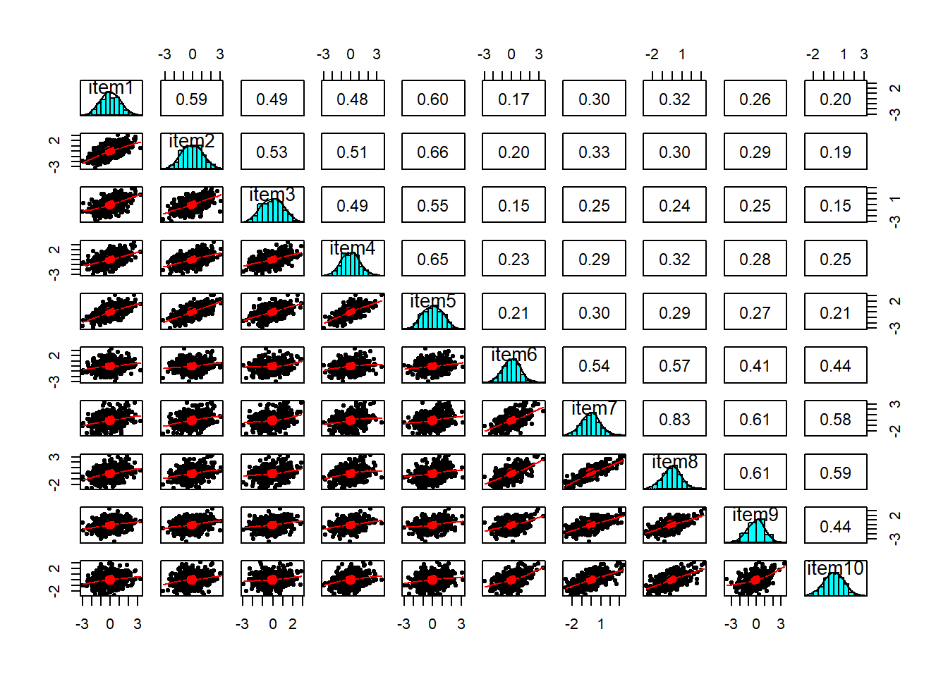
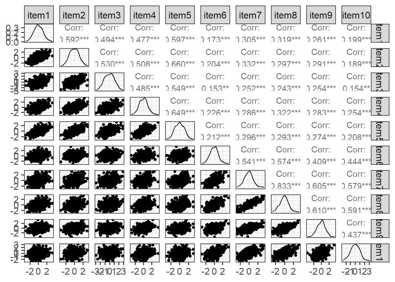
It also makes sense to check for linearity of relationships prior to conducting EFA. EFA is all based on correlations, which assume the relations we are capturing are linear.

You can check linearity of relations using pairs.panels(data) (also from psych), and you can view the histograms on the diagonals, allowing you to check univariate normality (which is usually a good enough proxy for multivariate normality).

Exercises: Conduct Problems

Data: Conduct Problems

A researcher is developing a new brief measure of Conduct Problems. She has collected data from n=450 adolescents on 10 items, which cover the following behaviours:

1. Stealing
2. Lying
3. Skipping school
4. Vandalism
5. Breaking curfew
6. Threatening others
7. Bullying
8. Spreading malicious rumours
9. Using a weapon
10. Fighting

Your task is to use the dimension reduction techniques you learned about in the lecture to help inform how to organise the items she has developed into subscales.

The data can be found at https://uoepsy.github.io/data/conduct_probs.csv

1. Check Suitability

Question A1

Read in the dataset from https://uoepsy.github.io/data/conduct_probs.csv.
The first column is clearly an ID column, and it is easiest just to discard this when we are doing factor analysis.

Create a correlation matrix for the items.
Inspect the items to check their suitability for exploratory factor analysis.

Solution

library(psych)
df <- read.csv("https://uoepsy.github.io/data/conduct_probs.csv")
# discard the first column
df <- df[,-1]

corr.test(df)  

Call:corr.test(x = df)
Correlation matrix 
       item1 item2 item3 item4 item5 item6 item7 item8 item9 item10
item1   1.00  0.59  0.49  0.48  0.60  0.17  0.30  0.32  0.26   0.20
item2   0.59  1.00  0.53  0.51  0.66  0.20  0.33  0.30  0.29   0.19
item3   0.49  0.53  1.00  0.49  0.55  0.15  0.25  0.24  0.25   0.15
item4   0.48  0.51  0.49  1.00  0.65  0.23  0.29  0.32  0.28   0.25
item5   0.60  0.66  0.55  0.65  1.00  0.21  0.30  0.29  0.27   0.21
item6   0.17  0.20  0.15  0.23  0.21  1.00  0.54  0.57  0.41   0.44
item7   0.30  0.33  0.25  0.29  0.30  0.54  1.00  0.83  0.61   0.58
item8   0.32  0.30  0.24  0.32  0.29  0.57  0.83  1.00  0.61   0.59
item9   0.26  0.29  0.25  0.28  0.27  0.41  0.61  0.61  1.00   0.44
item10  0.20  0.19  0.15  0.25  0.21  0.44  0.58  0.59  0.44   1.00
Sample Size 
[1] 450
Probability values (Entries above the diagonal are adjusted for multiple tests.) 
       item1 item2 item3 item4 item5 item6 item7 item8 item9 item10
item1      0     0     0     0     0     0     0     0     0      0
item2      0     0     0     0     0     0     0     0     0      0
item3      0     0     0     0     0     0     0     0     0      0
item4      0     0     0     0     0     0     0     0     0      0
item5      0     0     0     0     0     0     0     0     0      0
item6      0     0     0     0     0     0     0     0     0      0
item7      0     0     0     0     0     0     0     0     0      0
item8      0     0     0     0     0     0     0     0     0      0
item9      0     0     0     0     0     0     0     0     0      0
item10     0     0     0     0     0     0     0     0     0      0

 To see confidence intervals of the correlations, print with the short=FALSE option

cortest.bartlett(cor(df), n=450)

$chisq
[1] 2238

$p.value
[1] 0

$df
[1] 45

KMO(df)  

Kaiser-Meyer-Olkin factor adequacy
Call: KMO(r = df)
Overall MSA =  0.87
MSA for each item = 
 item1  item2  item3  item4  item5  item6  item7  item8  item9 item10 
  0.90   0.88   0.92   0.88   0.84   0.94   0.82   0.81   0.95   0.94 

pairs.panels(df)

or alternatively, if you want a ggplot based approach:

library(GGally)
ggpairs(data=df, diag=list(continuous="density"), axisLabels="show")

2. How many factors?

Question A2

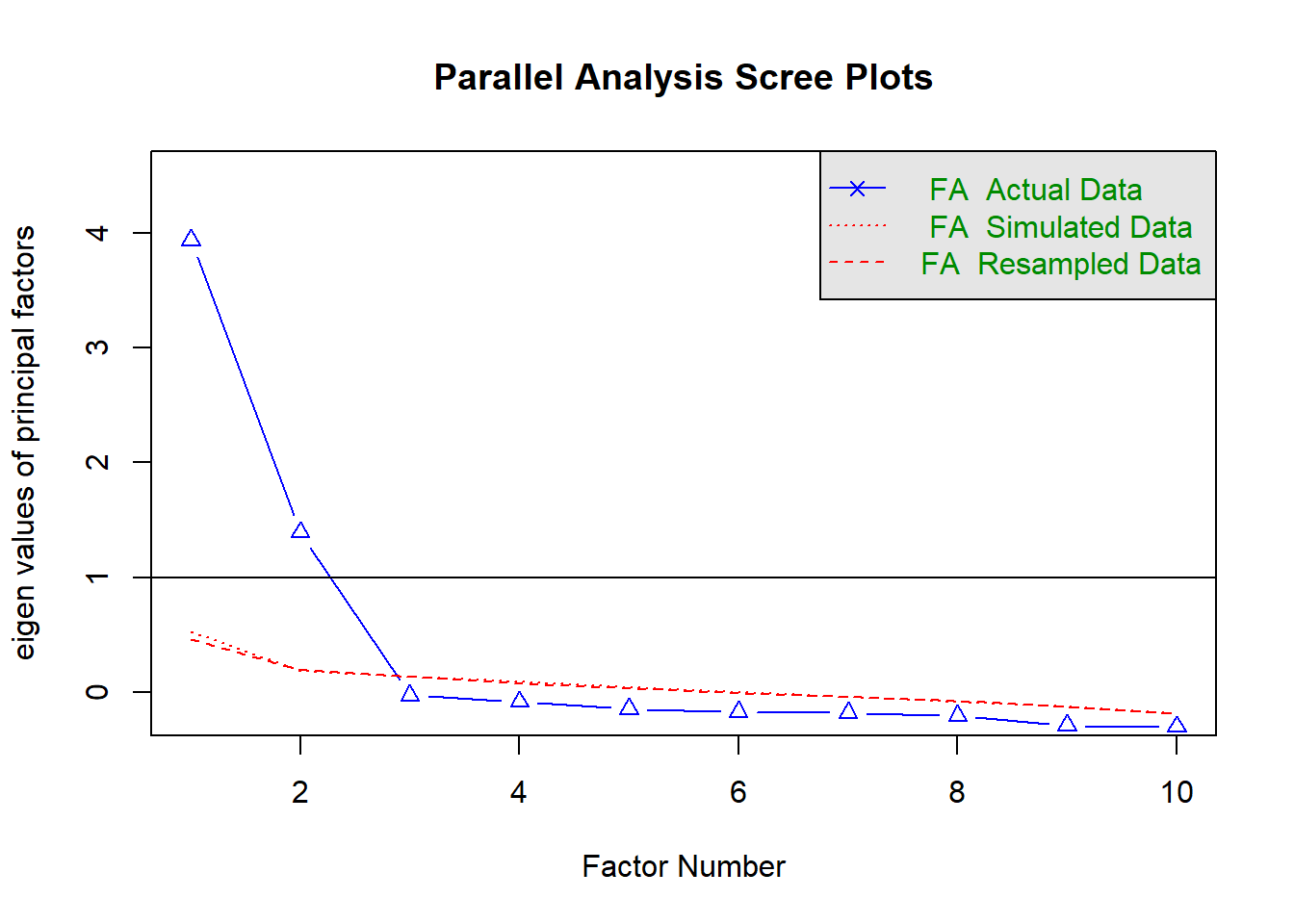
How many dimensions should be retained? This question can be answered in the same way as we did above for PCA.

Use a scree plot, parallel analysis, and MAP test to guide you.
You can use fa.parallel(data, fm = "fa") to conduct both parallel analysis and view the scree plot!

Solution

fa.parallel(df, fa = "fa")

Parallel analysis suggests that the number of factors =  2  and the number of components =  NA 

In this case the scree plot has a kink at the third factor, so we probably want to retain 2 factors.

We can conduct the MAP test using VSS(data).

VSS(df, plot = FALSE, n = ncol(df))$map

 [1] 0.1058 0.0338 0.0576 0.1035 0.1494 0.2520 0.3974 0.4552 1.0000     NA

The MAP test suggests retaining 2 factors.

3. Perform EFA

Now we need to perform the factor analysis. But there are two further things we need to consider, and they are:

1. whether we want to apply a rotation to our factor loadings, in order to make them easier to interpret, and
   
2. how do we want to extract our factors (it turns out there are loads of different approaches!).

Rotations?

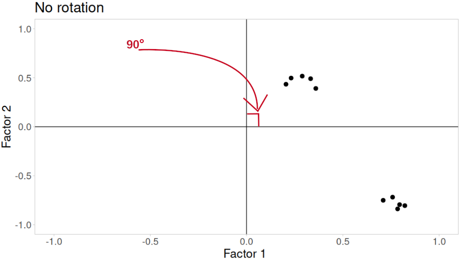
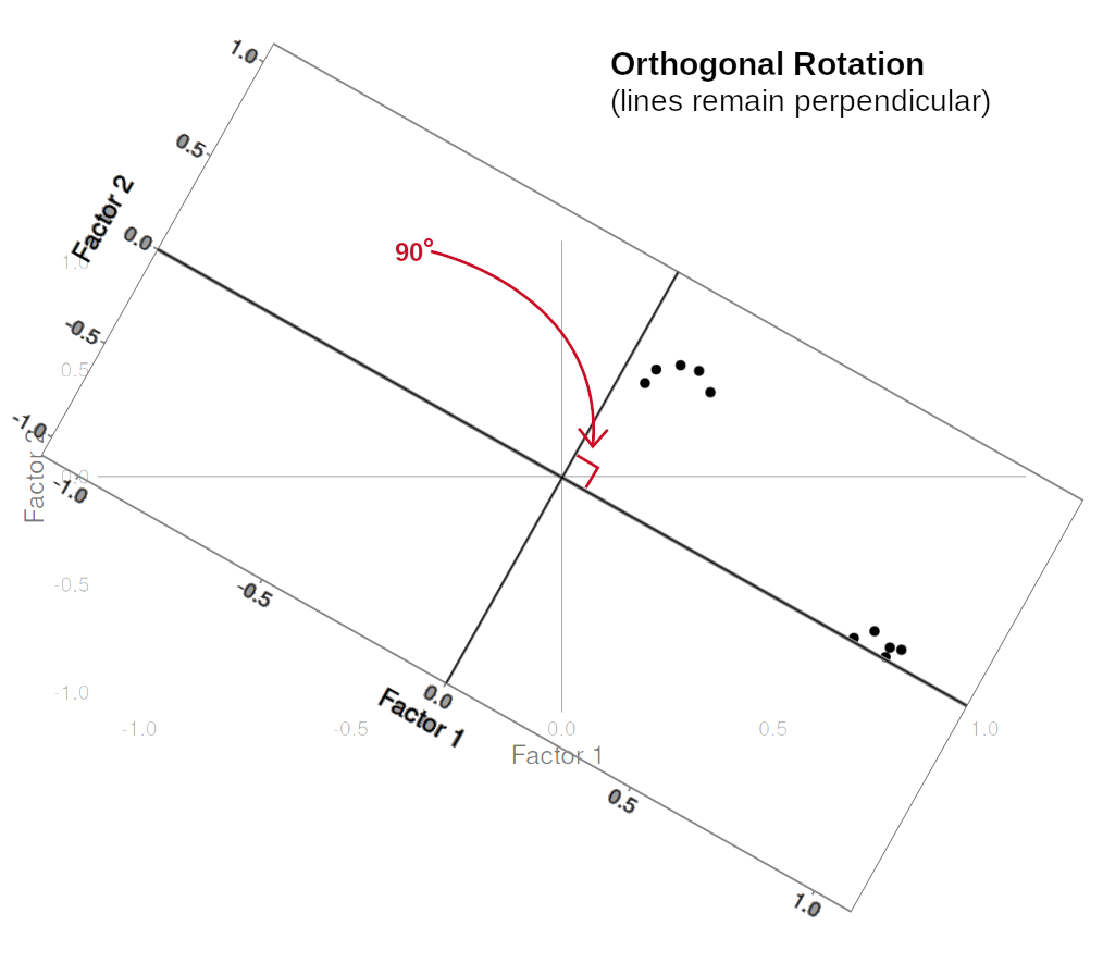
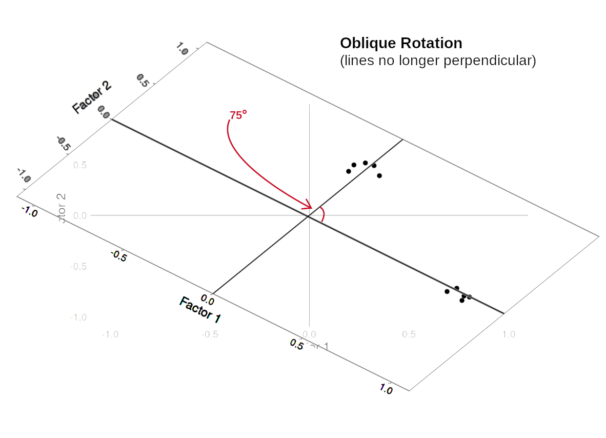
Rotations are so called because they transform our loadings matrix in such a way that it can make it more easy to interpret. You can think of it as a transformation applied to our loadings in order to optimise interpretability, by maximising the loading of each item onto one factor, while minimising its loadings to others. We can do this by simple rotations, but maintaining our axes (the factors) as perpendicular (i.e., uncorrelated) as in Figure 3, or we can allow them to be transformed beyond a rotation to allow the factors to correlate (Figure 4).

Figure 2: No rotation

Figure 3: Orthogonal rotation

Figure 4: Oblique rotation

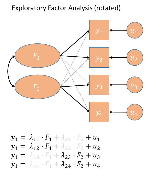
In our path diagram of the model (Figure 5), all the factor loadings remain present, but some of them become negligible. We can also introduce the possible correlation between our factors, as indicated by the curved arrow between \(F_1\) and \(F_2\).

Figure 5: Path diagrams for EFA with rotation

Factor Extraction

PCA (using eigendecomposition) is itself a method of extracting the different dimensions from our data. However, there are lots more available for factor analysis.

You can find a lot of discussion about different methods both in the help documentation for the fa() function from the psych package:

Factoring method fm=“minres” will do a minimum residual as will fm=“uls”. Both of these use a first derivative. fm=“ols” differs very slightly from “minres” in that it minimizes the entire residual matrix using an OLS procedure but uses the empirical first derivative. This will be slower. fm=“wls” will do a weighted least squares (WLS) solution, fm=“gls” does a generalized weighted least squares (GLS), fm=“pa” will do the principal factor solution, fm=“ml” will do a maximum likelihood factor analysis. fm=“minchi” will minimize the sample size weighted chi square when treating pairwise correlations with different number of subjects per pair. fm =“minrank” will do a minimum rank factor analysis. “old.min” will do minimal residual the way it was done prior to April, 2017 (see discussion below). fm=“alpha” will do alpha factor analysis as described in Kaiser and Coffey (1965)

And there are lots of discussions both in papers and on forums.

As you can see, this is a complicated issue, but when you have a large sample size, a large number of variables, for which you have similar communalities, then the extraction methods tend to agree. For now, don’t fret too much about the factor extraction method.²

Question A3

Use the function fa() from the psych package to conduct and EFA to extract 2 factors (this is what we suggest based on the various tests above, but you might feel differently - the ideal number of factors is subjective!). Use a suitable rotation (rotate = ?) and extraction method (fm = ?).

conduct_efa <- fa(data, nfactors = ?, rotate = ?, fm = ?)

Solution

For example, you could choose an oblimin rotation to allow factors to correlate and use minres as the extraction method.

conduct_efa <- fa(df, nfactors=2, rotate='oblimin', fm="minres")

4. Inspect

We can simply print the name of our model in order to see a lot of information. Let’s go through it in pieces.

Loadings

Factor Analysis using method =  minres
Call: fa(r = df, nfactors = 2, rotate = "oblimin", fm = "minres")
Standardized loadings (pattern matrix) based upon correlation matrix
         MR1   MR2   h2   u2 com
item1   0.03  0.71 0.52 0.48   1
item2   0.01  0.77 0.60 0.40   1
item3  -0.02  0.68 0.45 0.55   1
item4   0.06  0.68 0.50 0.50   1
item5  -0.04  0.87 0.73 0.27   1
item6   0.63 -0.02 0.39 0.61   1
item7   0.89  0.00 0.80 0.20   1
item8   0.92 -0.01 0.84 0.16   1
item9   0.63  0.09 0.45 0.55   1
item10  0.67 -0.03 0.43 0.57   1

Factor loading’s, like PCA loading’s, show the relationship of each measured variable to each factor. They range between -1.00 and 1.00 Larger absolute values represent stronger relationship between measured variable and factor.

• The columns that (depending upon estimation method) might be called MR/ML/PC are the factors. The number assigned to is arbitrary, and they might not always be in a numeric order (this has to do with a rotated solution). Typically, the numbering maps to how much variance each factor account for.
• h2: This is the “communality”, which is how much variance in the item is explained by the factors. It is calculated as the sum of the squared loadings.
  
• u2: This is \(1 - h2\). It is the residual variance, or the “uniqueness” for that item (i.e. the amount left unexplained).
  
• com: This is the “Item complexity”. It tells us how much a given item reflects a single factor (vs being “more complex” in that it represents multiple factors). It equals one if an item loads only on one factor, 2 if evenly loads on two factors, etc.

You can get these on their own using

conduct_efa$loadings

Variance Accounted For

                       MR1  MR2
SS loadings           2.92 2.80
Proportion Var        0.29 0.28
Cumulative Var        0.29 0.57
Proportion Explained  0.51 0.49
Cumulative Proportion 0.51 1.00

Below the factor loadings, we have a familiar set of measures of the variance in the data accounted for by each factor. This is very similar to what we saw with PCA.

• SS loadings: The sum of the squared loadings. The eigenvalues.
  
• Proportion Var: how much of the overall variance the factor accounts for out of all the variables.
• Cumulative Var: cumulative sum of Proportion Var.
• Proportion Explained: relative amount of variance explained (\(\frac{\text{Proportion Var}}{\text{sum(Proportion Var)}}\).
• Cumulative Proportion: cumulative sum of Proportion Explained.

You can get these on their own using

conduct_efa$Vaccounted

Factor Correlations

 With factor correlations of 
     MR1  MR2
MR1 1.00 0.43
MR2 0.43 1.00

Mean item complexity =  1

Whether we see this section will depend if we have run a factor analysis with \(\geq 2\) factors and a rotation.

• factor correlations: shows the correlation matrix between the factors.
• mean item complexity: shows the mean of the com column from the loadings above.

You can get these on their own using

conduct_efa$Phi

Tests, Fit Indices etc

We also get a whole load of other stuff that can sometimes be useful. These include: a test of an hypothesis that the 2 factors are sufficient; information on the number of observations; fit indices such as RMSEA, TLI RMSR etc; and measures of factor score adequacy (we’ll get to talking about factor scores next week).

Test of the hypothesis that 2 factors are sufficient.

The degrees of freedom for the null model are  45  and the objective function was  5.03 with Chi Square of  2238
The degrees of freedom for the model are 26  and the objective function was  0.09 

The root mean square of the residuals (RMSR) is  0.02 
The df corrected root mean square of the residuals is  0.02 

The harmonic number of observations is  450 with the empirical chi square  13.7  with prob <  0.98 
The total number of observations was  450  with Likelihood Chi Square =  40  with prob <  0.039 

Tucker Lewis Index of factoring reliability =  0.989
RMSEA index =  0.035  and the 90 % confidence intervals are  0.008 0.055
BIC =  -119
Fit based upon off diagonal values = 1
Measures of factor score adequacy             
                                                   MR1  MR2
Correlation of (regression) scores with factors   0.96 0.94
Multiple R square of scores with factors          0.92 0.88
Minimum correlation of possible factor scores     0.84 0.76

Question A4

Inspect the loadings (conduct_efa$loadings) and give the factors you extracted labels based on the patterns of loadings.

Look back to the description of the items, and suggest a name for your factors

Solution

You can inspect the loadings using:

print(conduct_efa$loadings, sort=TRUE)

Loadings:
       MR1    MR2   
item6   0.634       
item7   0.890       
item8   0.924       
item9   0.629       
item10  0.669       
item1          0.706
item2          0.772
item3          0.681
item4          0.676
item5          0.872

                MR1   MR2
SS loadings    2.90 2.784
Proportion Var 0.29 0.278
Cumulative Var 0.29 0.568

We can see that the first five items have high loadings for one factor and the second five items have high loadings for the other.

The first five items all have in common that they are non-aggressive forms of conduct problems, while the last five items are all aggressive behaviours. We could, therefore, label our factors: ‘non-aggressive’ and ‘aggressive’ conduct problems.

Question A5

How correlated are your factors?

We can inspect the factor correlations (if we used an oblique rotation) using:

conduct_efa$Phi

Solution

conduct_efa$Phi

     MR1  MR2
MR1 1.00 0.43
MR2 0.43 1.00

We can see here that there is a moderate correlation between the two factors. An oblique rotation would be appropriate here.

5. Write-up

Question A6

Drawing on your previous answers and conducting any additional analyses you believe would be necessary to identify an optimal factor structure for the 10 conduct problems, write a brief text that summarises your method and the results from your chosen optimal model.

Solution

The main principles governing the reporting of statistical results are transparency and reproducibility (i.e., someone should be able to reproduce your analysis based on your description).

An example summary would be:

First, the data were checked for their suitability for factor analysis. Normality was checked using visual inspection of histograms, linearity was checked through the inspection of the linear and lowess lines for the pairwise relations of the variables, and factorability was confirmed using a KMO test, which yielded an overall KMO of \(.87\) with no variable KMOs \(<.50\). An exploratory factor analysis was conducted to inform the structure of a new conduct problems test. Inspection of a scree plot alongside parallel analysis (using principal components analysis; PA-PCA) and the MAP test were used to guide the number of factors to retain. All three methods suggested retaining two factors; however, a one-factor and three-factor solution were inspected to confirm that the two-factor solution was optimal from a substantive and practical perspective, e.g., that it neither blurred important factor distinctions nor included a minor factor that would be better combined with the other in a one-factor solution. These factor analyses were conducted using minres extraction and (for the two- and three-factor solutions) an oblimin rotation, because it was expected that the factors would correlate. Inspection of the factor loadings and correlations reinforced that the two-factor solution was optimal: both factors were well-determined, including 5 loadings \(>|0.3|\) and the one-factor model blurred the distinction between different forms of conduct problems. The factor loadings are provided in Table 1³. Based on the pattern of factor loadings, the two factors were labelled ‘aggressive conduct problems’ and ‘non-aggressive conduct problems’. These factors had a correlation of \(r=.43\). Overall, they accounted for 57% of the variance in the items, suggesting that a two-factor solution effectively summarised the variation in the items.

Table 1: Factor Loadings

	MR1	MR2
item1		0.71
item2		0.77
item3		0.68
item4		0.68
item5		0.87
item6	0.63
item7	0.89
item8	0.92
item9	0.63
item10	0.67

PCA & EFA Comparison Exercise

Question A7

Using the same data, conduct a PCA using the principal() function.

What differences do you notice compared to your EFA?

Do you think a PCA or an EFA is more appropriate in this particular case?

Solution

We can use:

principal(df, nfactors=2)

Principal Components Analysis
Call: principal(r = df, nfactors = 2)
Standardized loadings (pattern matrix) based upon correlation matrix
        RC1  RC2   h2   u2 com
item1  0.17 0.77 0.62 0.38 1.1
item2  0.17 0.81 0.68 0.32 1.1
item3  0.11 0.75 0.58 0.42 1.0
item4  0.21 0.74 0.60 0.40 1.2
item5  0.16 0.85 0.75 0.25 1.1
item6  0.73 0.08 0.53 0.47 1.0
item7  0.87 0.20 0.80 0.20 1.1
item8  0.88 0.19 0.82 0.18 1.1
item9  0.72 0.21 0.56 0.44 1.2
item10 0.75 0.09 0.57 0.43 1.0

                       RC1  RC2
SS loadings           3.29 3.22
Proportion Var        0.33 0.32
Cumulative Var        0.33 0.65
Proportion Explained  0.51 0.49
Cumulative Proportion 0.51 1.00

Mean item complexity =  1.1
Test of the hypothesis that 2 components are sufficient.

The root mean square of the residuals (RMSR) is  0.06 
 with the empirical chi square  166  with prob <  1.9e-22 

Fit based upon off diagonal values = 0.98

We can see that while the loadings differ somewhat between the EFA and the PCA, the overall pattern is quite similar. This is not always the case, especially when the item communalities are low.

In terms of which method is more appropriate, arguably EFA would be more appropriate in this case because our researcher wishes to measure a theoretical construct (conduct problems), rather than simply reduce the dimensions of her data.

Footnotes

1. When we have some clear hypothesis about relationships between measured variables and latent factors, we might want to impose a specific factor structure on the data (e.g., items 1 to 10 all measure social anxiety, items 11 to 15 measure health anxiety, and so on). When we impose a specific factor structure, we are doing Confirmatory Factor Analysis (CFA). This is not covered in this course, but it’s important to note that in practice EFA is not wholly “exploratory” (your theory will influence the decisions you make) nor is CFA wholly “confirmatory” (in which you will inevitably get tempted to explore how changing your factor structure might improve fit).

2. (It’s a bit like the optimiser issue in the multi-level model block)

3. You should provide the table of factor loadings. It is conventional to omit factor loadings \(<|0.3|\); however, be sure to ensure that you mention this in a table note.