Analysis Example: Intervention

Each of these pages provides an analysis run through for a different type of design. Each document is structured in the same way:

• First the data and research context is introduced. For the purpose of these tutorials, we will only use examples where the data can be shared - either because it is from an open access publication, or because it is unpublished or simulated.
• Second, we go through any tidying of the data that is required, before creating some brief descriptives and visualizations of the raw data.
• Then, we conduct an analysis. Where possible, we translate the research questions into formal equations prior to fitting the models in lme4. Model comparisons are conducted, along with checks of distributional assumptions on our model residuals.
• Finally, we visualize and interpret our analysis.

Please note that there will be only minimal explanation of the steps undertaken here, as these pages are intended as example analyses rather than additional labs readings. Please also be aware that there are many decisions to be made throughout conducting analyses, and it may be the case that you disagree with some of the choices we make here. As always with these things, it is how we justify our choices that is important. We warmly welcome any feedback and suggestions to improve these examples: please email ug.ppls.stats@ed.ac.uk.

Overview

Intervention studies are where the researchers intervenes (e.g. through administration of a drug or treatment) as part of the study

The data used for this worked example are simulated to represent data from 50 participants, each measured at 3 different time-points (pre, during, and post) on a measure of stress. Half of the participants are in the control group, and half are in the treatment group (e.g. half received some cognitive behavioural therapy (CBT), half did not).

Code

set.seed(983)
library(tidyverse)
simMIX <- tibble(
  ppt = factor(rep(paste("ID", 1:50, sep=""),each=3)),
  ppt_int = rep(rnorm(50,0,15), each=3), 
  stress = round(
    c(rnorm(75,c(50,45,42),sd=c(5, 6, 5)),
      rnorm(75,c(55,30,20),sd=c(6, 10, 5))) + ppt_int,
    0),
  time = as_factor(rep(c("Pre", "During", "Post"), 50)),
  group = as_factor(c(rep("Control", 75), rep("Treatment", 75)))
) %>% select(-ppt_int)

Data Wrangling

Because we simulated our data, it is already nice and tidy. Each observation is a row, and we have variable indicating participant identifier (the ppt variable).

Code

summary(simMIX)

      ppt          stress           time          group   
 ID1    :  3   Min.   :-13.00   Pre   :50   Control  :75  
 ID10   :  3   1st Qu.: 29.00   During:50   Treatment:75  
 ID11   :  3   Median : 43.00   Post  :50                 
 ID12   :  3   Mean   : 42.22                             
 ID13   :  3   3rd Qu.: 55.75                             
 ID14   :  3   Max.   : 90.00                             
 (Other):132                                              

Code

bind_rows(head(simMIX), tail(simMIX))

# A tibble: 12 × 4
   ppt   stress time   group    
   <fct>  <dbl> <fct>  <fct>    
 1 ID1       65 Pre    Control  
 2 ID1       81 During Control  
 3 ID1       55 Post   Control  
 4 ID2       62 Pre    Control  
 5 ID2       57 During Control  
 6 ID2       67 Post   Control  
 7 ID49      58 Pre    Treatment
 8 ID49      34 During Treatment
 9 ID49      25 Post   Treatment
10 ID50      35 Pre    Treatment
11 ID50      21 During Treatment
12 ID50       0 Post   Treatment

Descriptives

We now have two factors of interest, scores over Time and by Group. So we do our descriptive statistics by multiple grouping factors.

Code

sumMIX <- 
  simMIX %>%
  group_by(time, group) %>%
  summarise(
    N = n_distinct(ppt),
    Mean = round(mean(stress, na.rm=T),2),
    SD = round(sd(stress, na.rm=T),2)
    )

Code

library(kableExtra)
kable(sumMIX) %>%
  kable_styling("striped")

time	group	N	Mean	SD
Pre	Control	25	52.84	14.60
Pre	Treatment	25	54.76	16.78
During	Control	25	49.64	13.23
During	Treatment	25	30.44	15.49
Post	Control	25	46.08	14.24
Post	Treatment	25	19.56	15.99

Visualizations

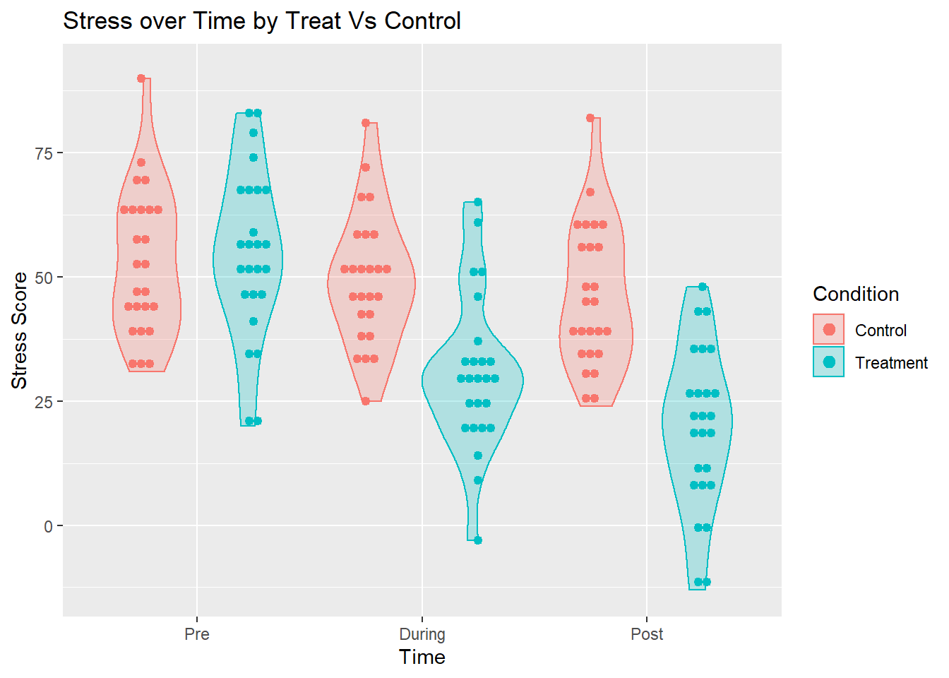
We can use a violin plot to visualize our data.

Code

simMIX %>% 
  ggplot(aes(x=time, y=stress, color=group, fill=group))  + 
  geom_violin(alpha = .25) + 
  geom_dotplot(binaxis='y', stackdir='center', position=position_dodge(1),
               dotsize = 0.5) +
  labs(x="Time", y = "Stress Score", 
       title="Stress over Time by Treat Vs Control", color="Condition", fill="Condition")

It is useful to note that the violin plot contains much of the same information that a more traditional boxplot would have, but provides more information on the actual distribution with groups as it draws on density plots.

What we can see here is that over time, the control group shows little change, but the treatment group shows distinct declines.
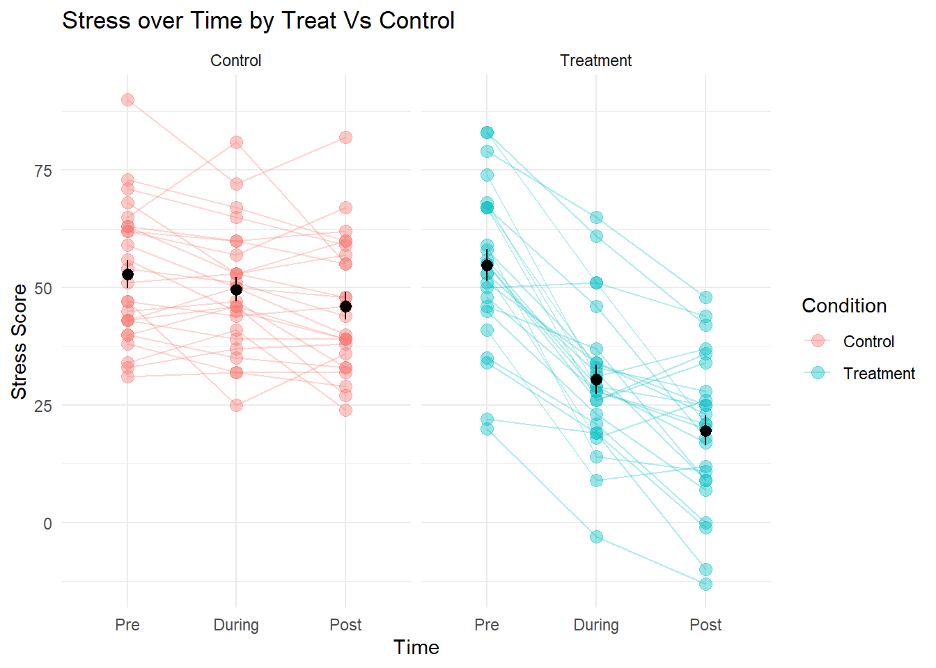
We can also consider line plots with separate facets for each condition:

Code

simMIX %>% 
  ggplot(aes(x=time, y=stress, col=group))  + 
  geom_point(size=3, alpha=.4)+
  geom_line(aes(group=ppt), alpha=.3)+
  stat_summary(geom="pointrange", col="black")+
  facet_wrap(~group)+
  labs(x="Time", y = "Stress Score", 
       title="Stress over Time by Treat Vs Control", color="Condition", fill="Condition")+
  theme_minimal()

Analysis

Equations

\[ \begin{aligned} \operatorname{stress}_{i[j]} &= \beta_{0i} + \beta_{1i}(\operatorname{timeDuring}_j) + \beta_{2i}(\operatorname{timePost}_j) + \varepsilon_{i[j]} \\ \beta_{0i} &= \gamma_{00} + \gamma_{01}(\operatorname{groupTreatment}_i) + \zeta_{0i} \\ \beta_{1i} &= \gamma_{10} + \gamma_{11}(\operatorname{groupTreatment}_i) \\ \beta_{2i} &= \gamma_{20} + \gamma_{21}(\operatorname{groupTreatment}_i) \\ & \text{for ppt i = 1,} \dots \text{, I} \end{aligned} \]

Fitting the models

Code

library(lme4)

Base model:

Code

m0 <- lmer(stress ~ 1 +
             (1 | ppt), data = simMIX)
summary(m0)

Linear mixed model fit by REML ['lmerMod']
Formula: stress ~ 1 + (1 | ppt)
   Data: simMIX

REML criterion at convergence: 1286.7

Scaled residuals: 
     Min       1Q   Median       3Q      Max 
-2.02099 -0.49670  0.01511  0.49445  1.96548 

Random effects:
 Groups   Name        Variance Std.Dev.
 ppt      (Intercept) 179.7    13.40   
 Residual             209.7    14.48   
Number of obs: 150, groups:  ppt, 50

Fixed effects:
            Estimate Std. Error t value
(Intercept)   42.220      2.234    18.9

Main effects:

Code

m1 <- lmer(stress ~ 1 + time + group +
             (1 | ppt), data = simMIX)
summary(m1)

Linear mixed model fit by REML ['lmerMod']
Formula: stress ~ 1 + time + group + (1 | ppt)
   Data: simMIX

REML criterion at convergence: 1185.9

Scaled residuals: 
     Min       1Q   Median       3Q      Max 
-1.69666 -0.62649  0.01574  0.59245  1.92387 

Random effects:
 Groups   Name        Variance Std.Dev.
 ppt      (Intercept) 166.57   12.91   
 Residual              98.01    9.90   
Number of obs: 150, groups:  ppt, 50

Fixed effects:
               Estimate Std. Error t value
(Intercept)      61.100      3.046  20.061
timeDuring      -13.760      1.980  -6.950
timePost        -20.980      1.980 -10.596
groupTreatment  -14.600      3.992  -3.657

Correlation of Fixed Effects:
            (Intr) tmDrng timPst
timeDuring  -0.325              
timePost    -0.325  0.500       
groupTrtmnt -0.655  0.000  0.000

Interaction:

Code

m2 <- lmer(stress ~ 1 + time + group + time*group +
             (1 | ppt), data = simMIX)
summary(m2)

Linear mixed model fit by REML ['lmerMod']
Formula: stress ~ 1 + time + group + time * group + (1 | ppt)
   Data: simMIX

REML criterion at convergence: 1096.5

Scaled residuals: 
     Min       1Q   Median       3Q      Max 
-1.83946 -0.53326 -0.05639  0.53766  2.31546 

Random effects:
 Groups   Name        Variance Std.Dev.
 ppt      (Intercept) 184.82   13.595  
 Residual              43.26    6.577  
Number of obs: 150, groups:  ppt, 50

Fixed effects:
                          Estimate Std. Error t value
(Intercept)                 52.840      3.020  17.494
timeDuring                  -3.200      1.860  -1.720
timePost                    -6.760      1.860  -3.634
groupTreatment               1.920      4.272   0.449
timeDuring:groupTreatment  -21.120      2.631  -8.028
timePost:groupTreatment    -28.440      2.631 -10.810

Correlation of Fixed Effects:
            (Intr) tmDrng timPst grpTrt tmDr:T
timeDuring  -0.308                            
timePost    -0.308  0.500                     
groupTrtmnt -0.707  0.218  0.218              
tmDrng:grpT  0.218 -0.707 -0.354 -0.308       
tmPst:grpTr  0.218 -0.354 -0.707 -0.308  0.500

Comparison with aov()

As we did with the simple repeated measures, we can also compare the sums of squares breakdown for the LMM (m2) by calling anova() on the lmer() model.

First with aov():

Code

m3 <- aov(stress ~ time + group + time*group +
            Error(ppt), data = simMIX)
summary(m3)

Error: ppt
          Df Sum Sq Mean Sq F value   Pr(>F)    
group      1   7993    7993   13.37 0.000633 ***
Residuals 48  28691     598                     
---
Signif. codes:  0 '***' 0.001 '**' 0.01 '*' 0.05 '.' 0.1 ' ' 1

Error: Within
           Df Sum Sq Mean Sq F value Pr(>F)    
time        2  11360    5680  131.31 <2e-16 ***
time:group  2   5452    2726   63.01 <2e-16 ***
Residuals  96   4153      43                   
---
Signif. codes:  0 '***' 0.001 '**' 0.01 '*' 0.05 '.' 0.1 ' ' 1

And then summarise:

Code

anova(m2)

Analysis of Variance Table
           npar  Sum Sq Mean Sq F value
time          2 11360.4  5680.2 131.305
group         1   578.5   578.5  13.373
time:group    2  5452.0  2726.0  63.014

For ease, lets compare all models with a parametric bootstrap likelihood ratio test:

Code

library(pbkrtest)
PBmodcomp(m1, m0)
PBmodcomp(m2, m1)

Bootstrap test; time: 58.26 sec; samples: 1000; extremes: 0;
large : stress ~ 1 + time + group + (1 | ppt)
stress ~ 1 + (1 | ppt)
         stat df   p.value    
LRT    90.348  3 < 2.2e-16 ***
PBtest 90.348     0.000999 ***
---
Signif. codes:  0 '***' 0.001 '**' 0.01 '*' 0.05 '.' 0.1 ' ' 1

Bootstrap test; time: 60.30 sec; samples: 1000; extremes: 0;
large : stress ~ 1 + time + group + time * group + (1 | ppt)
stress ~ 1 + time + group + (1 | ppt)
         stat df   p.value    
LRT    83.853  2 < 2.2e-16 ***
PBtest 83.853     0.000999 ***
---
Signif. codes:  0 '***' 0.001 '**' 0.01 '*' 0.05 '.' 0.1 ' ' 1

And extract some bootstrap 95% CIs

Code

confint(m2,method="boot")

                               2.5 %      97.5 %
.sig01                     11.063915  16.8989137
.sigma                      5.570576   7.3318954
(Intercept)                46.958215  58.9035049
timeDuring                 -6.598935  -0.1161317
timePost                  -10.473009  -3.1302747
groupTreatment             -7.001190  10.0517531
timeDuring:groupTreatment -26.395306 -16.1101659
timePost:groupTreatment   -33.665532 -23.2588741

Check Model

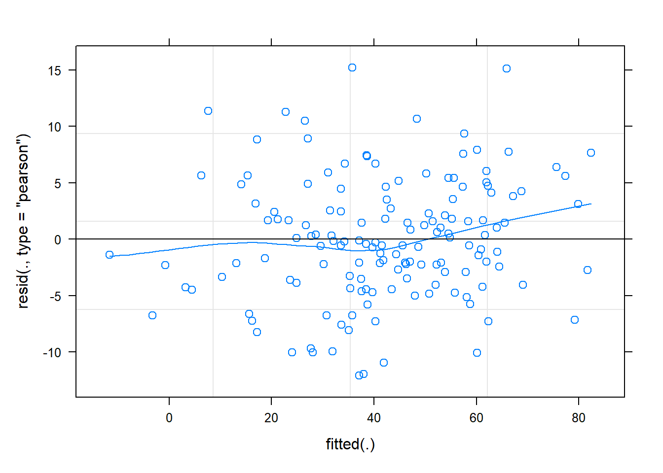
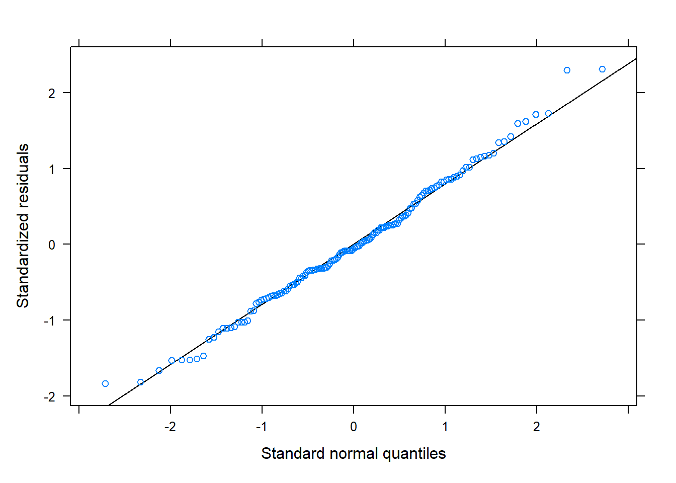
The residuals look reasonably normally distributed, and there seems to be fairly constant variance across the linear predictor. We might be a little concerned about the potential tails of the plot below, at which residuals don’t appear to have a mean of zero

Code

plot(m2, type = c("p","smooth"))

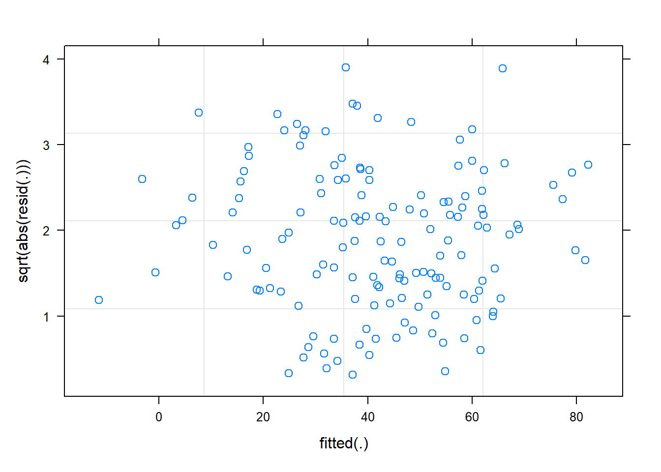
Code

plot(m2, sqrt(abs(resid(.)))~fitted(.))

Code

library(lattice)
qqmath(m2)

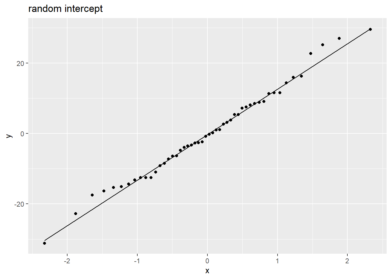
Random effects are (roughly) normally distributed:

Code

rans <- as.data.frame(ranef(m2)$ppt)
ggplot(rans, aes(sample = `(Intercept)`)) + 
  stat_qq() + stat_qq_line() +
  labs(title="random intercept")

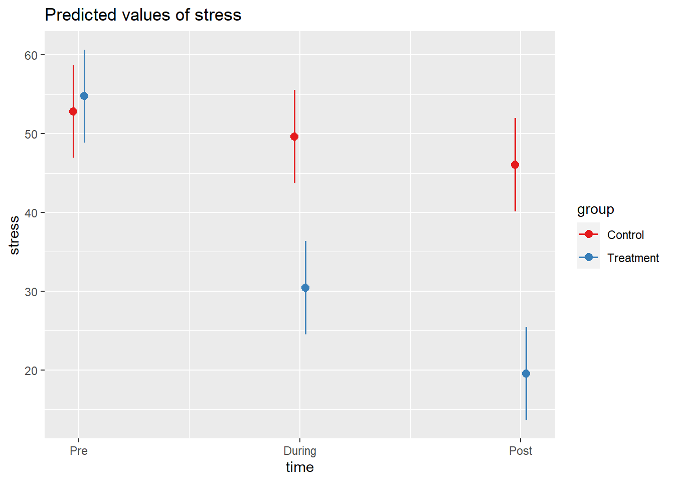
Visualise Model

Code

library(sjPlot)
plot_model(m2, type="int")

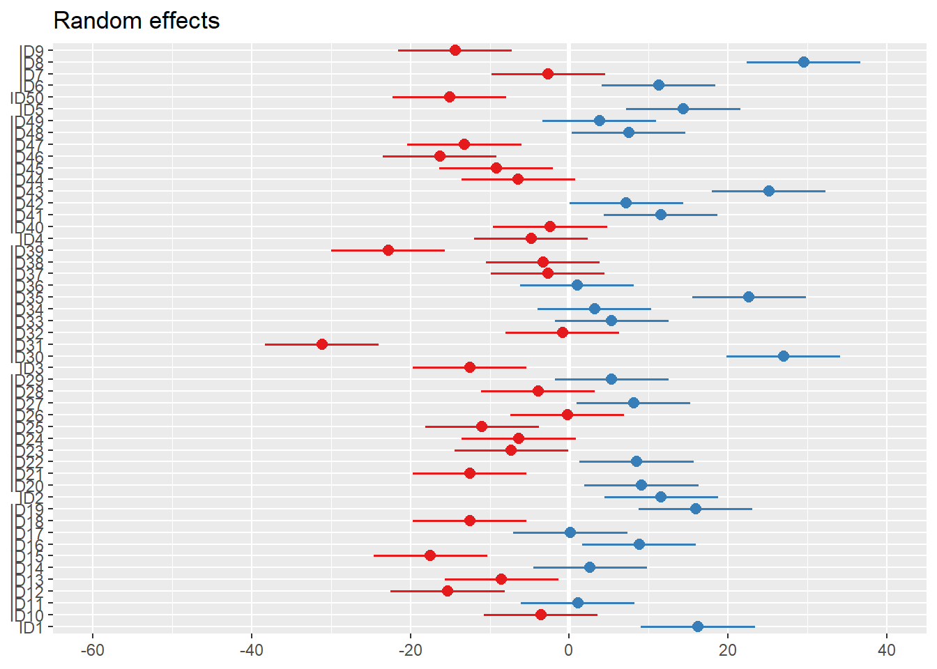
Code

plot_model(m2, type="re") # an alternative: dotplot.ranef.mer(ranef(m1))

Interpret model

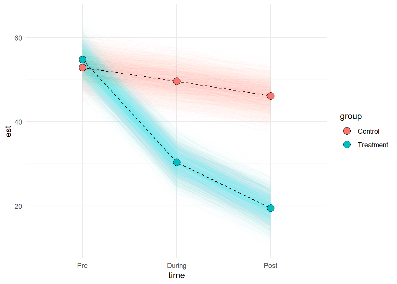
Stress at each study time-point (pre-, during- and post-intervention) was modeled using linear mixed effects models, with by-participant random intercepts, and the incremental addition of time, condition (control vs treatment) and their interaction. An interaction between time and condition improved model fit over the model without the interaction (Parametric bootstrap LRT 83.85, p < .001), suggesting that patterns of change over time in stress levels differed for the treatment group from the control group.
Result show that for the control group, stress did not show clear change between time-points 1 and 2 (-3.2, 95% CI [-6.92 – 0.32]), but by time-point 3 had reduced relative to time-point 1 by -6.76 [-10.58 – -3.3] points. Prior to the intervention (time-point 1), the treatment group did not appear to differ from the control group with respect to their level of stress, but showed an additional -21.12 [-26.75 – -15.63] point change by time-point 2 and -28.44 [-33.75 – -23.23] points by the end of the study (time-point 3). This pattern of results is shown in Figure 1.

Figure 1: Stress levels over time for control and treatment groups, with bootstrap prediction intervals (R = 2000)