Centering in MLM | Logistic MLM

Preliminaries

1. Create a new RMarkdown document or R script (whichever you like) for this week.

Centering & Scaling in LM

We have some data from a study investigating how perceived persuasiveness of a speaker is influenced by the rate at which they speak (you may remember this from the first report in DAPR2 last year!).

dap2 <- read_csv("https://uoepsy.github.io/data/dapr2_2122_report1.csv")

We can fit a simple linear regression (one predictor) to evaluate how speech rate (variable sp_rate in the dataset) influences perceived persuasiveness (variable persuasive in the dataset). There are various ways in which we can transform the predictor variable sp_rate, which in turn can alter the interpretation of some of our estimates:

Raw X

m1 <- lm(persuasive ~ sp_rate, data = dap2)
summary(m1)$coefficients

             Estimate Std. Error   t value     Pr(>|t|)
(Intercept) 55.532060  6.4016670  8.674625 6.848945e-15
sp_rate     -0.190987  0.4497113 -0.424688 6.716809e-01

The intercept and the coefficient for neuroticism are interpreted as:

• (Intercept): A audio clip of someone speaking at zero phones per second is estimated as having an average persuasive rating of 55.53.
  
• sp_rate: For every increase of one phone per second, perceived persuasiveness is estimated to decrease by -0.19.

Mean-Centered X

We can mean center our predictor and fit the model again:

dap2 <- dap2 %>% mutate(sp_rate_mc = sp_rate - mean(sp_rate))
m2 <- lm(persuasive ~ sp_rate_mc, data = dap2)
summary(m2)$coefficients

             Estimate Std. Error   t value     Pr(>|t|)
(Intercept) 52.874667  1.3519418 39.110165 6.429541e-80
sp_rate_mc  -0.190987  0.4497113 -0.424688 6.716809e-01

• (Intercept): A audio clip of someone speaking at the mean phones per second is estimated as having an average persuasive rating of 52.87.
  
• sp_rate_mc: For every increase of one phone per second, perceived persuasiveness is estimated to decrease by -0.19.

Standardised X

We can standardise our predictor and fit the model yet again:

dap2 <- dap2 %>% mutate(sp_rate_z = scale(sp_rate))
m3 <- lm(persuasive ~ sp_rate_z, data = dap2)
summary(m3)$coefficients

             Estimate Std. Error   t value     Pr(>|t|)
(Intercept) 52.874667   1.351942 39.110165 6.429541e-80
sp_rate_z   -0.576077   1.356471 -0.424688 6.716809e-01

• (Intercept): A audio clip of someone speaking at the mean phones per second is estimated as having an average persuasive rating of 52.87.
  
• sp_rate_z: For every increase of one standard deviation in phones per second, perceived persuasiveness is estimated to decrease by -0.58.

Remember that the scale(sp_rate) is subtracting the mean from each value, then dividing those by the standard deviation. The standard deviation of dap2$sp_rate is:

sd(dap2$sp_rate)

[1] 3.016315

so in our variable dap2$sp_rate_z, a change of 3.02 gets scaled to be a change of 1 (because we are dividing by sd(dap2$sp_rate)).

coef(m1)[2] * sd(dap2$sp_rate)

  sp_rate 
-0.576077 

coef(m3)[2]

sp_rate_z 
-0.576077 

Note that these models are identical. When we conduct a model comparison between the 3 models, the residual sums of squares is identical for all models:

anova(m1,m2,m3)

Analysis of Variance Table

Model 1: persuasive ~ sp_rate
Model 2: persuasive ~ sp_rate_mc
Model 3: persuasive ~ sp_rate_z
  Res.Df   RSS Df Sum of Sq F Pr(>F)
1    148 40576                      
2    148 40576  0         0         
3    148 40576  0         0         

What changes when you center or scale a predictor in a standard regression model (one fitted with lm())?

• The variance explained by the predictor remains exactly the same
• The intercept will change to be the estimated mean outcome where that predictor is “0”. Scaling and centering changes what “0” represents, thereby changing this estimate (the significance test will therefore also change because the intercept now has a different meaning)
• The slope of the predictor will change according to any scaling (e.g. if you divide your predictor by 10, the slope will multiply by 10).
• The test of the slope of the predictor remains exactly the same.

Exercises: Centering in the MLM

Data: Hangry

The study is interested in evaluating whether hunger influences peoples’ levels of irritability (i.e., “the hangry hypothesis”), and whether this is different for people following a diet that includes fasting. 81 participants were recruited into the study. Once a week for 5 consecutive weeks, participants were asked to complete two questionnaires, one assessing their level of hunger, and one assessing their level of irritability. The time and day at which participants were assessed was at a randomly chosen hour between 7am and 7pm each week. 46 of the participants were following a five-two diet (five days of normal eating, 2 days of fasting), and the remaining 35 were following no specific diet.

The data are available at: https://uoepsy.github.io/data/hangry.csv.

variable	description
q_irritability	Score on irritability questionnaire (0:100)
q_hunger	Score on hunger questionnaire (0:100)
ppt	Participant
fivetwo	Whether the participant follows the five-two diet

Question 1

Read carefully the description of the study above, and try to write out (in lmer syntax) an appropriate model to test the research aims.
e.g.:

outcome ~ explanatory variables + (???? | grouping)

Try to think about the maximal random effect structure (i.e. everything that can vary by-grouping is estimated as doing so).

To help you think through the steps to get from a description of a research study to a model specification, think about your answers to the following questions.

Q: What is our outcome variable?

Hint: The research is looking at how hunger influences irritability, and whether this is different for people on the fivetwo diet.

Q: What are our explanatory variables?

Hint: The research is looking at how hunger influences irritability, and whether this is different for people on the fivetwo diet.

Q: Is there any grouping (or “clustering”) of our data that we consider to be a random sample? If so, what are the groups?

Hint: We can split our data in to groups of each participant. We can also split it into groups of each diet. Which of these groups have we randomly sampled? Do we have a random sample of participants? Do we have a random sample of diets? Another way to think of this is “if i repeated the experiment, what these groups be different?”

Solution

Our outcome is irritability here, because it is the thing that we are trying to explain through peoples’ hunger levels and diets.

lmer(irritability ~  explanatory variables + (???? | grouping))

We are interested in the effect of hunger on irritability, and whether this effect is different for the five-two diet. So we are interested in the interaction:

lmer(irritability ~  hunger + diet + hunger:diet + (???? | grouping))

(remember that hunger + diet + hunger:diet is just a more explicit way of writing hunger*diet).

If we did this experiment again, would we have different participants?
Yes. If we did this experiment again, would we have different diets? No, because we’re interested in the specific differences between the five-two diet and no dieting. This means we will likely want to by-participant random deviations (e.g. the ( ... | participant) bit in lmer). But we won’t have by-diet random effects (1 | diet) because the diet differences are the specific differences that we wish to test.

lmer(irritability ~  hunger + diet + hunger:diet + (???? | participant))

Thinking about what can be modelled as randomly varying between participants, we have some options:

1. participants vary in how irritable they are on average
   (the intercept, 1 | participant)
2. participants vary in how much hunger influences their irritability
   (the effect of hunger, hunger | participant)
3. participants vary in how much diet influences irritability
   (the effect of diet, diet | participant)
4. participants vary in how much diet effects hunger’s influence on irritability
   (the interaction between diet and hunger, diet:hunger | participant)

We can vary 1 and 2, but not 3 and 4. This is because each participant is either following the five-two diet or they are not. So for a single participant, we can’t assess “the effect diet has” on anything, because we haven’t seen that participant under different diets. if we try to plot a single participants’ data, we can see that it is impossible for us to assess “the effect of diet”:

By contrast, we can vary the intercept and the effect of hunger, because each participant has multiple values of irritability, and multiple different observations of hunger. We can think about a single participant’s “effect of hunger on irritability” and how we might fit a line to their data:

lmer(irritability ~  hunger + diet + hunger:diet + (1 + hunger | participant))

Total, Within, Between

Recall our research aim:

… whether hunger influences peoples’ levels of irritability (i.e., “the hangry hypothesis”), and whether this is different for people following a diet that includes fasting.

Forgetting about any differences due to diet, let’s just think about the relationship between irritability and hunger. How should we interpret this research aim?
Was it:

1. “Are people more irritable if they are, on average, more hungry than other people?”
   
2. “Are people more irritable if they are, for them, more hungry than they usually are?”
   
3. Some combination of both a. and b.

This is just one demonstration of how the statistical methods we use can constitute an integral part of our development of a research project, and part of the reason that data analysis for scientific cannot be so easily outsourced after designing the study and collecting the data.

As our data currently is currently stored, the relationship between irritability and the raw scores on the hunger questionnaire q_hunger represents some ‘total effect’ of hunger on irritability. This is a bit like interpretation c. above - it’s a composite of both the ‘within’ ( b. ) and ‘between’ ( a. ) effects. The problem with this is that the ‘total effect’ isn’t necessarily all that meaningful. It may tell us that ‘being higher on the hunger questionnaire is associated with being more irritable’, but how can we apply this information? It is not specifically about the comparison between hungry people and less hungry people, and nor is it about how person i changes when they are more hungry than usual. It is both these things smushed together.

To disaggregate the ‘within’ and ‘between’ effects of hunger on irritability, we can group-mean center. For ‘between’, we are interested in how irritability is related to the average hunger levels of a participant, and for ‘within’, we are asking how irritability is related to a participants’ relative levels of hunger (i.e., how far above/below their average hunger level they are.).

Question 2

Add to the data these two columns:

1. a column which contains the average hungriness score for each participant.
2. a column which contains the deviation from each person’s hunger score to that person’s average hunger score.

Hint: You’ll find group_by() %>% mutate() very useful here.

Solution

hangry <- 
    hangry %>% group_by(ppt) %>%
        mutate(
            avg_hunger = mean(q_hunger),
            hunger_gc = q_hunger - avg_hunger
        )
head(hangry)

# A tibble: 6 × 6
# Groups:   ppt [2]
  q_irritability q_hunger ppt   fivetwo avg_hunger hunger_gc
           <dbl>    <dbl> <chr> <fct>        <dbl>     <dbl>
1             17       30 N1p1  1             26.6     3.4  
2             19       27 N1p1  1             26.6     0.400
3             19       29 N1p1  1             26.6     2.4  
4             20       33 N1p1  1             26.6     6.4  
5             24       14 N1p1  1             26.6   -12.6  
6             30       28 N1p2  1             32.6    -4.6  

Question 3

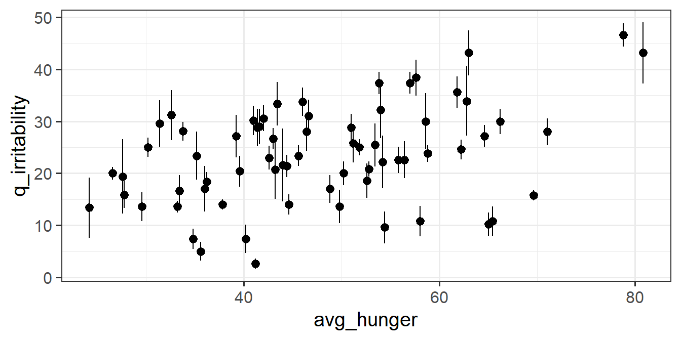
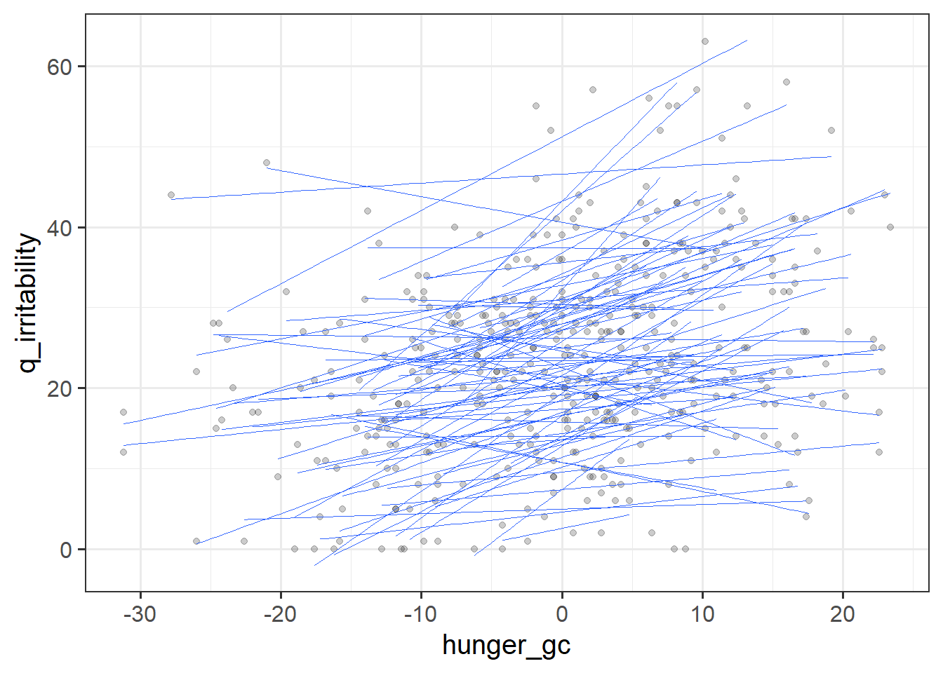
For each of the new variables you just added, plot the irritability scores against those variables.

• Does it look like hungry people are more irritable than less hungry people?
  
• Does it look like when people are more hungry than normal, they are more irritable?

Solution

We might find it easier to look at a plot where each participant is represented as their mean plus an indication of their range of irritability scores:

ggplot(hangry,aes(x=avg_hunger,y=q_irritability))+
    stat_summary(geom="pointrange")

There appears to be a slight positive relationship between a persons’ average hunger and their irritability scores.

It is harder to tell what the relationship is between participant-centered hunger and irritability, because there are a lot of different lines (one for each participant). To make it easier to get an idea of what’s happening, we’ll make the plot fit a simple lm() (a straight line) for each participants’ data:

ggplot(hangry,aes(x=hunger_gc,y=q_irritability, group=ppt))+
  geom_point(alpha = .2) + 
  geom_smooth(method=lm, se=FALSE, lwd=.2)

I think there might be a positive trend in here, in that participants tend to be higher irritability when they are higher (for them) on the hunger score.

Question 4

We have taken the raw hunger scores and separated them into two parts (raw hunger scores = participants’ average hunger score + observation level deviations from those averages), that represent two different aspects of the relationship between hunger and irritability.

Adjust your model specification to include these two separate variables as predictors, instead of the raw hunger scores.

Hints:

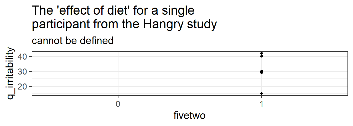
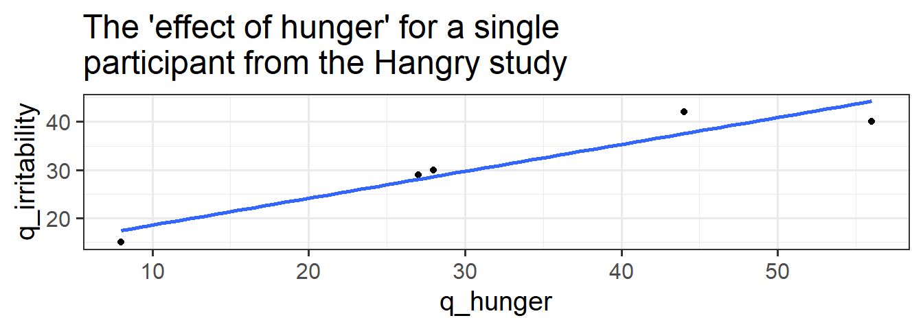
• hunger * diet could be replaced by (hunger1 + hunger2) * diet, thereby allowing each aspect of hunger to interact with diet.
• We can only put one of these variables in the random effects (1 + hunger | participant). Recall that above we discussed how we cannot have (diet | participant), because “an effect of diet” makes no sense for a single participant (they are either on the diet or they are not, so there is no ‘effect’). Similarly, each participant has only one value for their average hungriness.

Solution

library(lme4)
hangrywb <- lmer(q_irritability ~ (avg_hunger + hunger_gc)* fivetwo + 
                (1 + hunger_gc | ppt), 
                data = hangry,
                control = lmerControl(optimizer="bobyqa"))

Question 5

Hopefully, you have fitted a model similar to the below:

hangrywb <- lmer(q_irritability ~ (avg_hunger + hunger_gc) * fivetwo + 
                (1 + hunger_gc | ppt), data = hangry,
            control = lmerControl(optimizer="bobyqa"))

Below, we have obtained p-values using the Satterthwaite Approximation of \(df\) for the test of whether the fixed effects are zero, so we can see the significance of each estimate.

Provide an answer for each of these questions:

1. For those following no diet, is there evidence to suggest that people who are on average more hungry are more irritable?
2. Is there evidence to suggest that this is different for those following the five-two diet? In what way?
3. Do people following no diet tend to be more irritable when they are more hungry than they usually are?
4. Is there evidence to suggest that this is different for those following the five-two diet? In what way?
5. (Trickier:) What does the fivetwo coefficient represent?

term	Estimate	Std. Error	df	t value	Pr(>|t|)
(Intercept)	17.131	5.15	77	3.33	0.0013
avg_hunger	0.004	0.11	77	0.04	0.9708
hunger_gc	0.186	0.08	65.4	2.46	0.0167
fivetwo1	-10.855	6.54	77	-1.66	0.1008
avg_hunger:fivetwo1	0.466	0.13	77	3.49	<0.001
hunger_gc:fivetwo1	0.381	0.1	68.5	3.76	<0.001

Solution

1: For those following no diet, is there evidence to suggest that people who are on average more hungry are more irritable?
A: ‘No diet’ is the reference level of the five-two variable, and because we have an interaction, that means the avg_hunger coefficient will provide the relevant estimate. There is no evidence (\(p>.05\)) to suggest that when not dieting, hungrier people are more irritable than less hungry people.

2: Is there evidence to suggest that this is different for those following the five-two diet? In what way?
A: This is the interaction between avg_hunger:fivetwo1. We can see that, for every increase of 1 in average hunger, irritability is estimated to increase by 0.47 more for those in the five-two diet than it does for those following no diet.
These units are still in terms of the original scale (i.e. 0 to 100).

3: Do people following no diet tend to be more irritable when they are more hungry than they usually are? A: This is the estimate for the coefficient of hunger_gc. For people following no diet, there is an estimated 0.19 increase in irritability for every 1 unit more hungry they become.

4: Is there evidence to suggest that this is different for those following the five-two diet? In what way? A: This effect of a 1 unit change on within-person hunger increasing irritability is increased for those who are following the five-two diet by an additional 0.38

5: What does the fivetwo1 coefficient represent? A: This represents the group difference of irritability between those on the five-two diet vs those not dieting, for someone who has an average hunger score of 0.

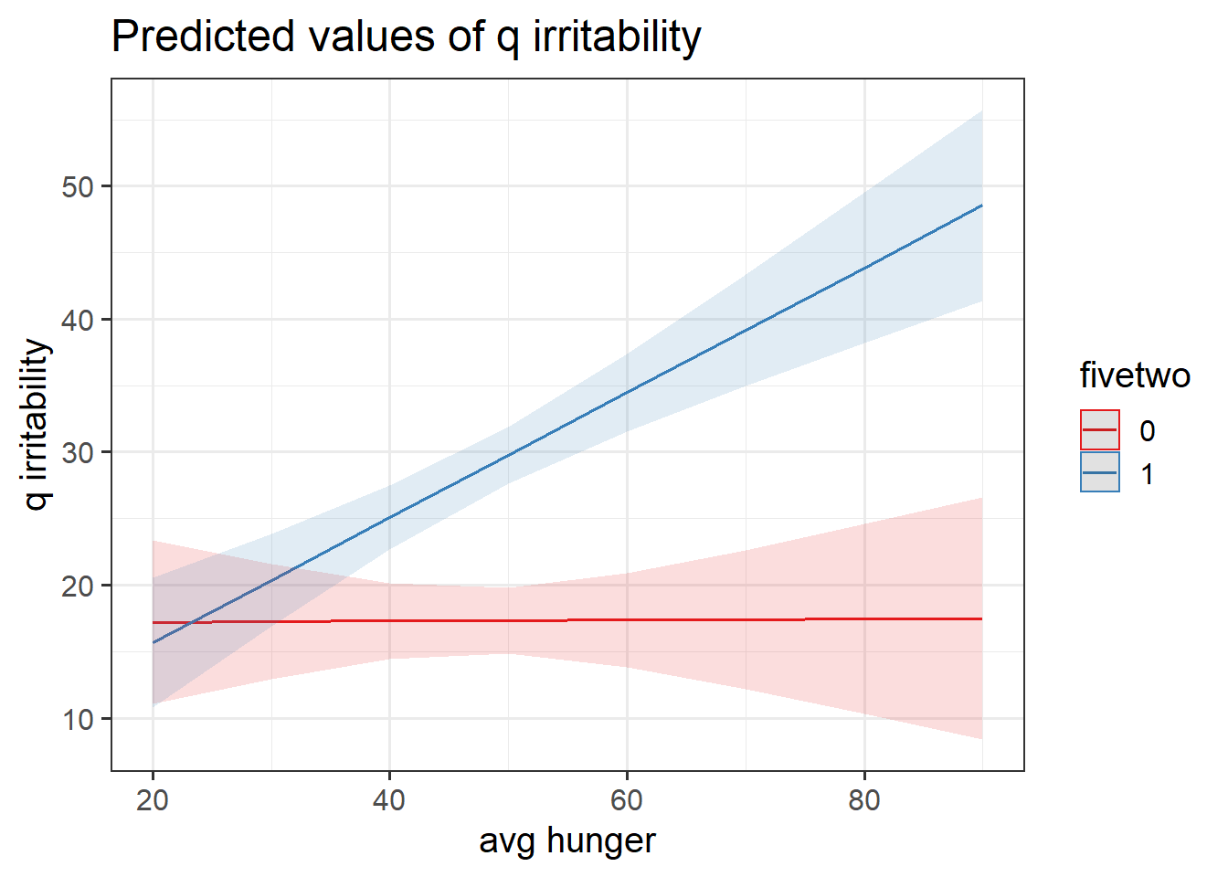
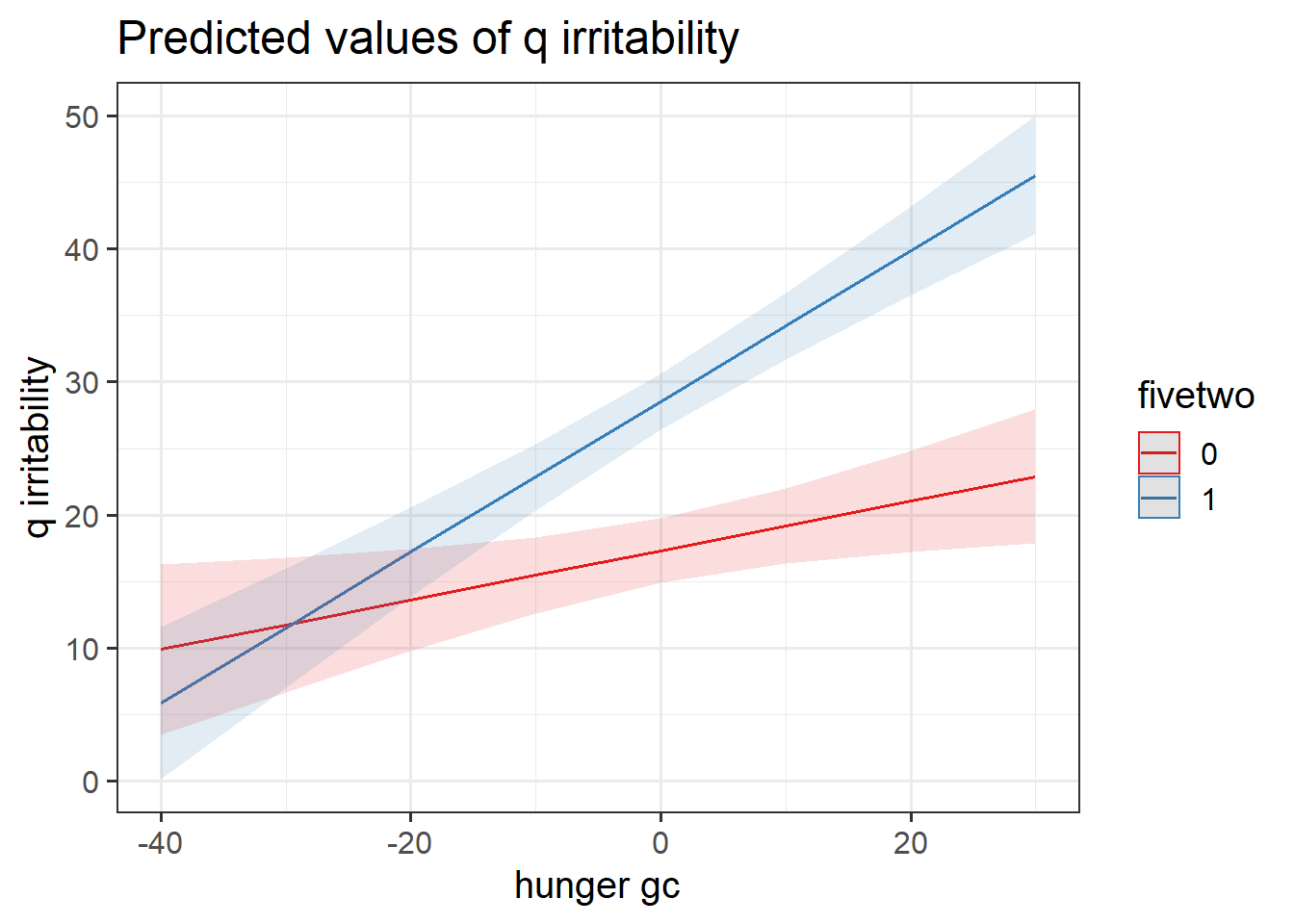
Question 6

Construct two plots showing the two model estimated interactions. Think about your answers to the previous question, and check that they match with what you are seeing in the plots (do not underestimate the utility of this activity for helping understanding!).

Hint: This isn’t as difficult as it sounds. the sjPlot package can do it in one line of code!

Solution

library(sjPlot)
plot_model(hangrywb, type = "int")[[1]]

We saw in the model coefficients that for the reference level of fivetwo, the “No Diet” group, there was no association between how hungry a person is on average and their irritability. This is the red line we see in the plot above. We also saw the interaction avg_hunger:fivetwo1 indicates that irritability is estimated to increase by 0.47 more for those in the five-two diet than it does for those following no diet. So the blue line is should be going up more steeply than the red line (which is flat). And it is!

plot_model(hangrywb, type = "int")[[2]]

From the coefficient of hunger_gc we get the estimated amount by which irritability increases for every 1 more hungry that a person becomes (when they’re on “No Diet”). This is the slope of the red line. The interaction hunger_gc:fivetwo1 gave us the adjustment to get from the red line to the blue line. It is positive and significant, which matches with the fact that the blue line is clearly steeper in this plot.

Question 7

Load the lmerTest package and fit the model again. Take a look at the summary - you should now have the \(df\), \(t\)-value, and \(p\)-value for each estimate.

Write-up the results.

Solution

library(lmerTest)
hangrywb2 <- lmer(q_irritability ~ (avg_hunger + hunger_gc)* fivetwo + 
                (1 + hunger_gc | ppt), 
                data = hangry,
                REML = TRUE,
                control = lmerControl(optimizer="bobyqa"))
summary(hangrywb2)

Linear mixed model fit by REML. t-tests use Satterthwaite's method [
lmerModLmerTest]
Formula: 
q_irritability ~ (avg_hunger + hunger_gc) * fivetwo + (1 + hunger_gc |  
    ppt)
   Data: hangry
Control: lmerControl(optimizer = "bobyqa")

REML criterion at convergence: 2734.8

Scaled residuals: 
     Min       1Q   Median       3Q      Max 
-2.41378 -0.59064 -0.04539  0.54264  2.39536 

Random effects:
 Groups   Name        Variance Std.Dev. Corr 
 ppt      (Intercept) 48.0827  6.9342        
          hunger_gc    0.1451  0.3809   -0.01
 Residual             23.3050  4.8275        
Number of obs: 405, groups:  ppt, 81

Fixed effects:
                      Estimate Std. Error         df t value Pr(>|t|)    
(Intercept)          17.130959   5.146478  76.999477   3.329 0.001341 ** 
avg_hunger            0.003863   0.105327  76.998524   0.037 0.970835    
hunger_gc             0.185773   0.075601  65.409225   2.457 0.016659 *  
fivetwo1            -10.854713   6.535684  76.999696  -1.661 0.100813    
avg_hunger:fivetwo1   0.465897   0.133539  76.998690   3.489 0.000806 ***
hunger_gc:fivetwo1    0.381412   0.101393  68.486392   3.762 0.000352 ***
---
Signif. codes:  0 '***' 0.001 '**' 0.01 '*' 0.05 '.' 0.1 ' ' 1

Correlation of Fixed Effects:
            (Intr) avg_hn hngr_g fivtw1 avg_:1
avg_hunger  -0.971                            
hunger_gc   -0.002  0.000                     
fivetwo1    -0.787  0.765  0.002              
avg_hngr:f1  0.766 -0.789  0.000 -0.968       
hngr_gc:fv1  0.002  0.000 -0.746 -0.002  0.000

To investigate the association between irritability and hunger, and whether this relationship is different depending on whether or not participants are on a restricted diet such as the five-two, a multilevel linear model was fitted.
To disaggregate between the differences in irritability due to people being in general more/less hungry, and those due to people being more/less hungry than usual for them, irritability was regressed onto both participants’ average hunger scores their relative hunger levels. Both of these were allowed to interact with whether or not participants were on the five-two diet. Random intercepts and slopes of relative-hunger level were included for participants. The model was fitting with restricted maximum likelihood estimation with the lme4 package (Bates et al., 2015), using the bobyqa optimiser from the lme4. \(P\)-values were obtained using the Satterthwaite approximation for degrees of freedom.

Results indicate that for people on no diet, being more hungry than normal was associated with greater irritability (\(\beta = 0.186,\ SE = 0.08,\ t(65.4) = 2.46,\ p = 0.0167\)), and that this was increased for those following the five-two diet (\(\beta = 0.381,\ SE = 0.1,\ t(68.5) = 3.76,\ p <0.001\)). Although for those not on a specific diet there was no evidence for an association between irritability and being generally a more hungry person (\(p = 0.9708\)), there a significant interaction was found between average hunger and being on the five-two diet (\(\beta = 0.466,\ SE = 0.13,\ t(77) = 3.49,\ p <0.001\)), suggesting that when dieting, hungrier people tend to be more irritable than less hungry people.
Results suggest that the ‘hangry hypothesis’ may occur within people (when a person is more hungry than they usually are, they tend to be more irritable), but not necessarily between hungry/less hungry people. Dieting was found to increase the association for both between-hunger and within-hunger with irritability.

Other within-group transformations

As well as within-group mean centering a predictor (like we have done above). There are quite a few similar things we can do, for which the logic is the same.

For instance, we can within-group standardise a predictor. This would disagregate within and between effects, but interpretation would of the within effect would be the estimated change in \(y\) associated with being 1 standard deviation higher in \(x\) for that group.

We can also do within-group transformations on our outcome variable. This allows to address questions such as:

“Are people more irritable than they usually are (\(y\) is group-mean centered) if they are, for them, more hungry than they usually are (\(x\) is group-mean centered)?”

Optional Exercises: Logistic MLM

Don’t forget to look back at other materials!

Back in DAPR2, we introduced logistic regression in semester 2, week 8. The lab contained some simulated data based on a hypothetical study about inattentional blindness. That content will provide a lot of the groundwork for this week, so we recommend revisiting it if you feel like it might be useful.

lmer() >> glmer()

Remember how we simply used glm() and could specify the family = "binomial" in order to fit a logistic regression? Well it’s much the same thing for multi-level models!

• Gaussian model: lmer(y ~ x1 + x2 + (1 | g), data = data)
  
• Binomial model: glmer(y ~ x1 + x2 + (1 | g), data = data, family = binomial(link='logit'))
  • or just glmer(y ~ x1 + x2 + (1 | g), data = data, family = "binomial")
  • or glmer(y ~ x1 + x2 + (1 | g), data = data, family = binomial)

Binary? Binomial?

For binary regression, all the data in our outcome variable has to be a 0 or a 1.
For example, the correct variable below:

participant	question	correct
1	1	1
1	2	0
1	3	1
...	...	...

But we can re-express this information in a different way, when we know the total number of questions asked.

participant	questions_correct	questions_incorrect
1	2	1
2	1	2
3	3	0
...	...	...

To model data when it is in this form, we can express our outcome as cbind(questions_correct, questions_incorrect)

Memory Recall & Finger Tapping

Research Question: After accounting for effects of sentence length, does the rhythmic tapping of fingers aid memory recall?

Researchers recruited 40 participants. Each participant was tasked with studying and then recalling 10 randomly generated sentences between 1 and 14 words long. For 5 of these sentences, participants were asked to tap their fingers along with speaking the sentence in both the study period and in the recall period. For the remaining 5 sentences, participants were asked to sit still.
The data are available at https://uoepsy.github.io/data/memorytap.csv, and contains information on the length (in words) of each sentence, the condition (static vs tapping) under which it was studied and recalled, and whether the participant was correct in recalling it.

variable	description
ppt	Participant Identifier (n=40)
slength	Number of words in sentence
condition	Condition under which sentence is studied and recalled ('static' = sitting still, 'tap' = tapping fingers along to sentence)
correct	Whether or not the sentence was correctly recalled

Question 8 (Optional)

Research Question: After accounting for effects of sentence length, does the rhythmic tapping of fingers aid memory recall?

Fit an appropriate model to answer the research question.

Hint:

• our outcome is conceptually ‘memory recall’, and it’s been measured by “Whether or not a sentence was correctly recalled”. This is a binary variable.
  
• we have multiple observations for each ?????
  This will define our ( | ??? ) bit

Solution

memtap <- read_csv("https://uoepsy.github.io/data/memorytap.csv")

When we fit the maximal model, note that we obtain a singular fit. The variance of the slength effect between participants is quite small relative to the others, and there is a correlation between it and the random intercepts.

tapmod <- glmer(correct ~ 1 + slength + condition + 
                  (1 + slength + condition | ppt),
      data = memtap,
      family = binomial)
isSingular(tapmod)

[1] TRUE

VarCorr(tapmod)

 Groups Name         Std.Dev. Corr         
 ppt    (Intercept)  1.032849              
        slength      0.070307 -1.000       
        conditiontap 0.665626  0.590 -0.590

let’s remove the random effect of slength | ppt.

tapmod2 <- glmer(correct ~ 1 + slength + condition + 
                  (1 + condition | ppt),
      data = memtap,
      family = binomial)

the model now looks a bit better (not a singular fit):

summary(tapmod2)

Generalized linear mixed model fit by maximum likelihood (Laplace
  Approximation) [glmerMod]
 Family: binomial  ( logit )
Formula: correct ~ 1 + slength + condition + (1 + condition | ppt)
   Data: memtap

     AIC      BIC   logLik deviance df.resid 
   537.6    561.5   -262.8    525.6      394 

Scaled residuals: 
    Min      1Q  Median      3Q     Max 
-1.8949 -0.8955  0.4483  0.7962  1.6862 

Random effects:
 Groups Name         Variance Std.Dev. Corr
 ppt    (Intercept)  0.2755   0.5249       
        conditiontap 0.4207   0.6486   0.66
Number of obs: 400, groups:  ppt, 40

Fixed effects:
             Estimate Std. Error z value Pr(>|z|)  
(Intercept)   0.76140    0.37077   2.054   0.0400 *
slength      -0.12086    0.04721  -2.560   0.0105 *
conditiontap  0.50945    0.24317   2.095   0.0362 *
---
Signif. codes:  0 '***' 0.001 '**' 0.01 '*' 0.05 '.' 0.1 ' ' 1

Correlation of Fixed Effects:
            (Intr) slngth
slength     -0.890       
conditiontp -0.154 -0.029

Take some time to remind yourself from DAPR2 of the interpretation of logistic regression coefficients.

In family = binomial(link='logit'), we are modelling the log-odds. We can obtain estimates on this scale using:

• fixef(model)
• summary(model)$coefficients
• tidy(model) from broom.mixed
  
• (there are probably more ways, but I can’t think of them right now!)

We can use exp(), to get these back into odds and odds ratios.

Question 9 (Optional)

Interpret each of the fixed effect estimates from your model.

Solution

fixef(tapmod2)

 (Intercept)      slength conditiontap 
   0.7613976   -0.1208591    0.5094460 

exp(fixef(tapmod2))

 (Intercept)      slength conditiontap 
   2.1412669    0.8861589    1.6643689 

• (Intercept): For an sentence with zero words, when sitting statically, the odds of correctly recalling the sentence are 2.14. This is equivalent to a \(\frac{2.14}{1 + 2.14} = 0.6815287\) probability of getting it correct.
  
• slength: After accounting for differences due to tapping/not-tapping during study & recall, for every 1 word longer a sentence is, the odds of correctly recalling the sentence is decreased by 0.89.
• conditiontap: After accounting for differences in recall due to sentence length, finger tapping during the study and recall of sentences was associated with 1.66 increased odds correct recall in comparison to sitting still.

Question 10 (Optional)

Checking the assumptions in non-gaussian models in general (i.e. those where we set the family to some other error distribution) can be a bit tricky, and this is especially true for multilevel models.

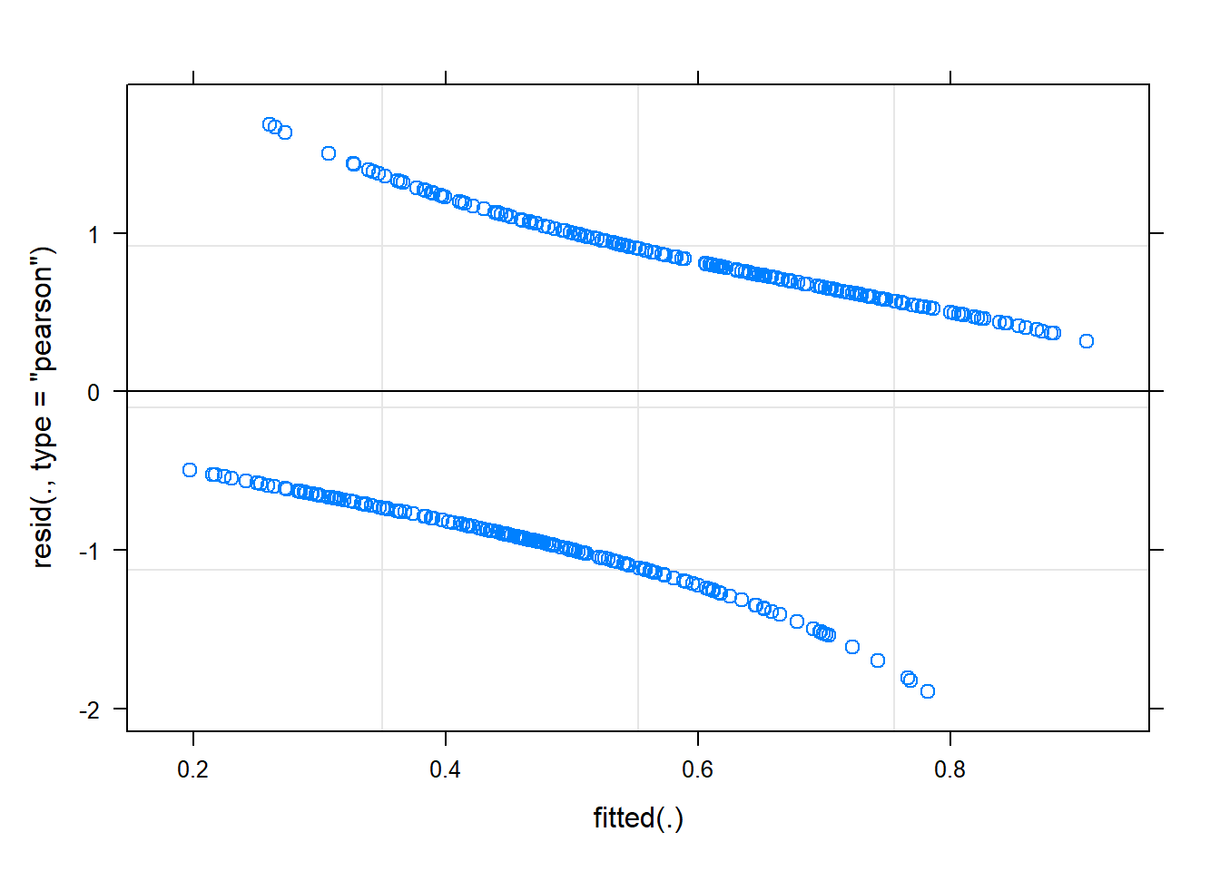
For the logistic MLM, the standard assumptions of normality etc for our Level 1 residuals residuals(model) do not hold. However, it is still useful to quickly plot the residuals and check that \(|residuals|\leq 2\) (or \(|residuals|\leq 3\) if you’re more relaxed). We don’t need to worry too much about the pattern though.

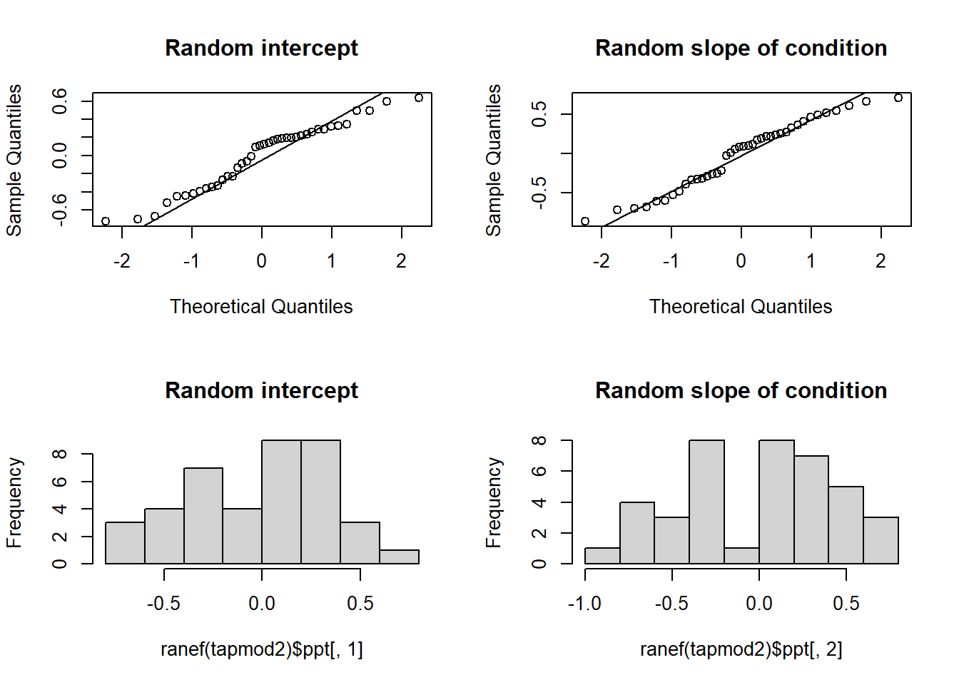
While we’re more relaxed about Level 1 residuals, we do still want our random effects ranef(model) to look fairly normally distributed.

1. Plot the level 1 residuals and check whether any are greater than 3 in magnitude
2. Plot the random effects (the level 2 residuals) and assess the normality.

for beyond DAPR3

• The HLMdiag package doesn’t support diagnosing influential points/clusters for glmer, but there is a package called influence.me which might help: https://journal.r-project.org/archive/2012/RJ-2012-011/RJ-2012-011.pdf
• There are packages which aim to create more interpretable residual plots for these models via simulation, such as the DHARMa package: https://cran.r-project.org/web/packages/DHARMa/vignettes/DHARMa.html

Solution

plot(tapmod2)

sum(abs(resid(tapmod2))>3)

[1] 0

All residuals are between -3 and 3.

The random effects look okay here. Not perfect, but bear in mind we have only 40 participants.

qqnorm(ranef(tapmod2)$ppt[, 1], main = "Random intercept")
qqline(ranef(tapmod2)$ppt[, 1])
qqnorm(ranef(tapmod2)$ppt[, 2], main = "Random slope of condition")
qqline(ranef(tapmod2)$ppt[, 2])
hist(ranef(tapmod2)$ppt[, 1])
hist(ranef(tapmod2)$ppt[, 2])