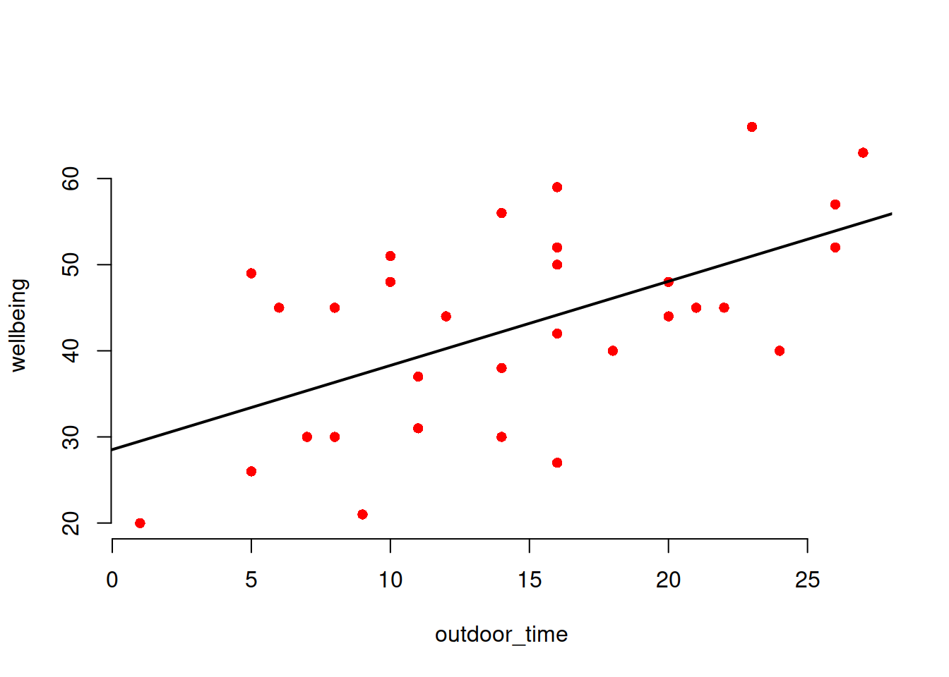
Fitting the following regression model which predicts wellbeing from the time spent outdoors
\[
\text{wellbeing}_i
= \beta_0
+ \beta_1 \ \text{outdoor_time}_i
+ \epsilon_i
\]
results in the following fitted line:
In simple linear regression, we defined our model through a number of components:
\(\beta_0\) / \(b_0\) / “the intercept.”
This is the predicted wellbeing when an individual spends 0 hours outdoors
It is where the regression line cuts the y-axis when x = 0.
It is the estimated expected value of \(y\) when \(x = 0\).
\(\beta_1\) / \(b_1\) / “the coefficient of \(\text{wellbeing}\).”
This is the predicted increase in the average wellbeing for every additional hour of outdoor time.
It is the estimated expected increase in \(y\) for a one-unit increase in \(x\).
\(\epsilon\) / \(e\) / “the residuals” or “error term.”
Represents the deviations from the actual values to the model-predicted values. The standard deviation of all these gets denoted \(\sigma\).
In the plot above, these are the vertical distances from each red dot to the black line.
Multiple linear regression
When we extended this to multiple regression, we essentially just added more explanatory variables, meaning we fitted more coefficients.
The values of \(y\) are now modelled as some relationship of more than just one \(x\) variable. In the case of two predictors, denote these by \(x_1\) and \(x_2\) respectively.
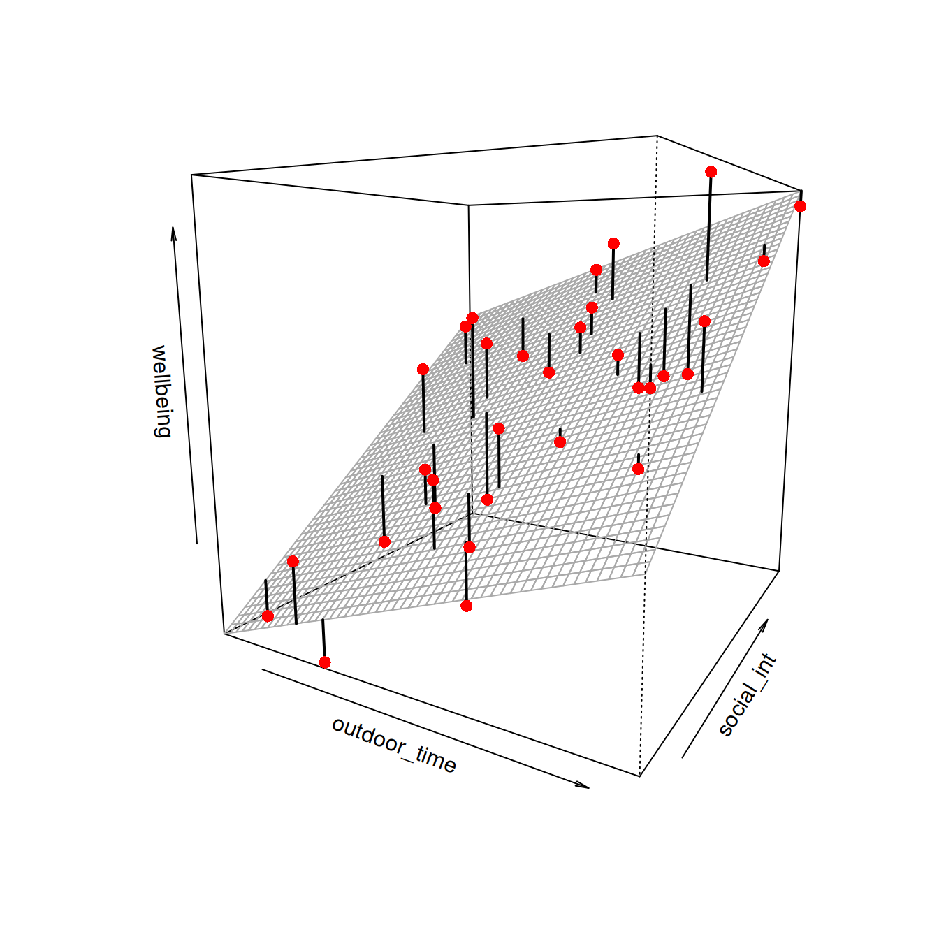
In the plot below with two predictors, we would have a slope for each predictor. Each coefficient represents the gradient of the regression surface along each dimension.
Interactions
We then saw how we can let the relationships between the outcome \(y\) and an explanatory variable \(x_1\) vary as a function of some other explanatory variable \(x_2\).
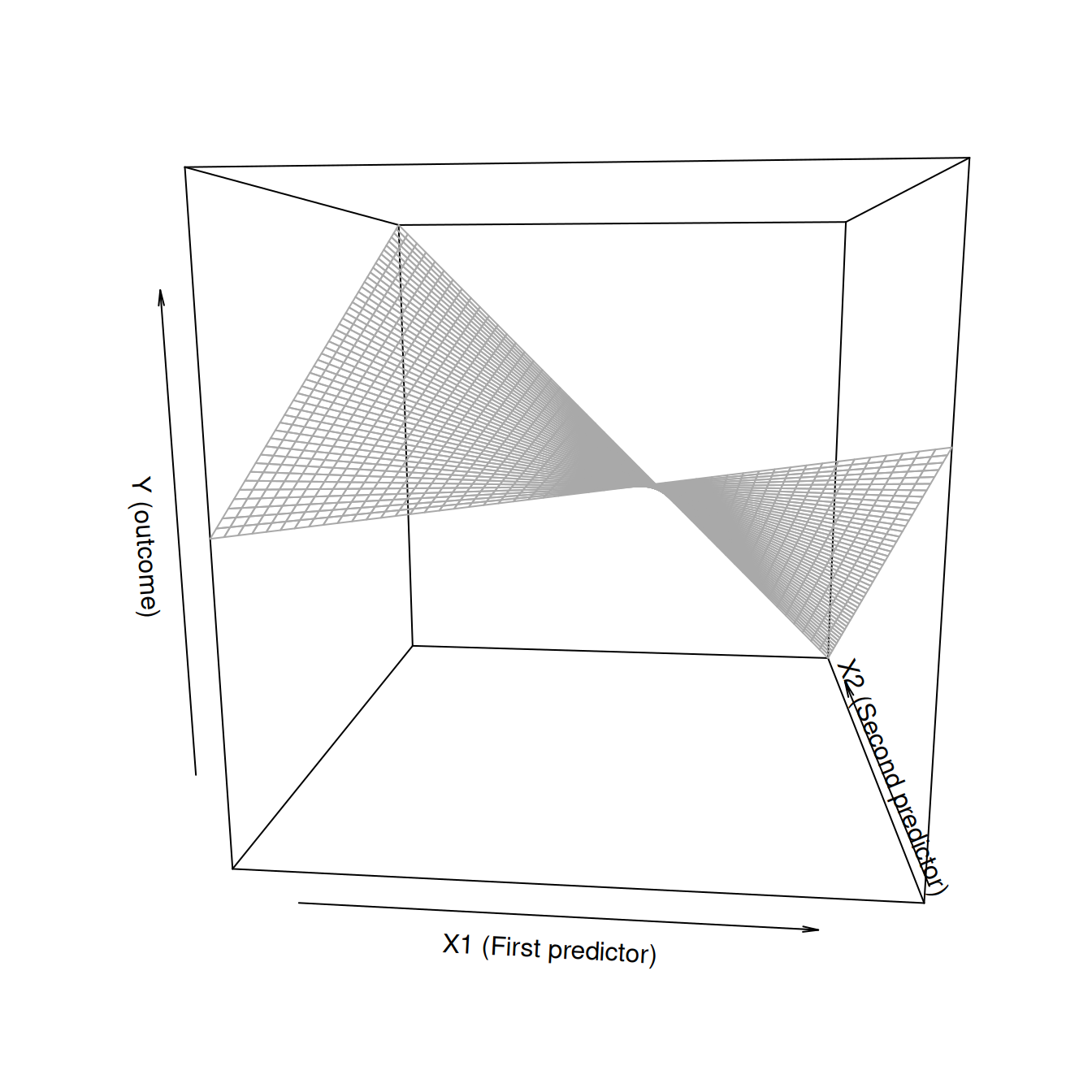
In the plot below, if someone asks you “what is the relationship between \(x_1\) and \(x\), your reply should (hopefully) be”well, it depends on what the value of \(x_2\) is"
This is captured in the curvature of the regression surface below, and we estimate it with a combination of 3 coefficients:
\(\beta_1\): the effect of \(x_1\) on \(y\) where \(x_2=0\)
(this is the slope of the surface where it meets the front face of the cube)
\(\beta_2\): the effect of \(x_2\) on \(y\) where \(x_1=0\)
(this is the slope of the surface where it meets the left of face of the cube)
\(\beta_3\): the amount to which (1) and (2) are adjusted when there is an increase in the other variable.
Categorical explanatory variables
Throughout these, we also saw how this applied when we had explanatory variables that were categorical.
They were entered in to the model as a set of “dummy variables” (zeroes and ones), representing differences between groups. If we had a categorical variable which contained \(k\) levels (or “groups,” or “categories”), then we R will put \(k-1\) dummy variables into the model for us, and we will get out \(k-1\) coefficients.
The default behaviour in R is that, depending on what we set as our reference level, the coefficients represent the difference from this group to each of the others.
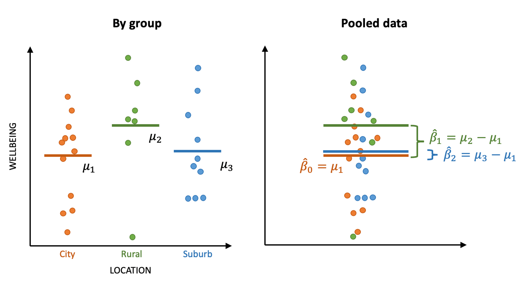
In the plots below, if “City” is the reference, then the coefficient locationRural would represent the vertical distance from the red line to the green line, and the coefficient locationSuburb would be the vertical distance from the red line to the blue line.
Note - because categorical predictors are coded as various dummy variables of zeroes and ones, the assumption of linearity is intrinsically there. The only possible way to get from the red line to the green line is via a straight line.
ANOVA & categorical interactions
A linear model summary tells you whether each of the difference between the mean of the \(i\)th group from the reference group mean is significant or not, e.g. \(\hat \beta_1 = \mu_2 - \mu_1\), \(\hat \beta_2 = \mu_3 - \mu_1\), \(\hat \beta_4 = \mu_3 - \mu_1\), and so on.
So, if you have \(k\) groups, you will have \(k-1\) such differences.
For the wellbeing example, we have 2 such differences (while the intercept is the mean for the reference group):
wb_mdl <- lm(wellbeing ~ location, data = mwdata)
summary(wb_mdl)
##
## Call:
## lm(formula = wellbeing ~ location, data = mwdata)
##
## Residuals:
## Min 1Q Median 3Q Max
## -28.571 -6.325 2.164 7.000 20.900
##
## Coefficients:
## Estimate Std. Error t value Pr(>|t|)
## (Intercept) 41.000 3.008 13.629 3.87e-14 ***
## locationRural 7.571 5.333 1.420 0.166
## locationSuburb 1.100 4.756 0.231 0.819
## ---
## Signif. codes: 0 '***' 0.001 '**' 0.01 '*' 0.05 '.' 0.1 ' ' 1
##
## Residual standard error: 11.65 on 29 degrees of freedom
## Multiple R-squared: 0.06759, Adjusted R-squared: 0.003291
## F-statistic: 1.051 on 2 and 29 DF, p-value: 0.3625
What if your question was not “Does the mean of group 3 differ from the mean of group 1?” which is answered by looking at the model summary()?
Say your question was “Does location impact wellbeing?” or “Is there a difference in wellbeing across the diffrent locations?”
This does not specify one specific location, but rather concerns checking whether there was a difference overall - that is, whether the mean wellbeing for city, rural and suburb are all equal or at least two differ.
This is where ANOVA comes in, which is run via anova(<fitted model>) and we have an F-test and the corresponding p-value.
anova(wb_mdl)
## Analysis of Variance Table
##
## Response: wellbeing
## Df Sum Sq Mean Sq F value Pr(>F)
## location 2 285.4 142.69 1.0512 0.3625
## Residuals 29 3936.6 135.75
The first row tells us that the factor outdoor_time is not statistically significant, meaning that there is not enough evidence to reject the null hypothesis that the mean wellbeing is the same among the three different locations.
We just said that anova() returns a row for each predictor, testing whether the estimated mean response (wellbeing) differs among the three groups – that is, whether the mean response differs among the possible values of the predictor (location).
What if the predictor does not represent groups, but a continuous variable?
The idea is the same! Basically, we are testing whether at each \(x\) value the estimated mean \(y\) is the same. Imagine increasing the number of groups to really many… In other words, we are testing whether the line is flat, meaning that the predictor has no influence on the response.
Binary data
How do we proceed if we want to perform a similar analysis to linear regression but for a response variable which is not numeric?
Consider the following questions:
What features of speech influence the likelihood of an utterance being perceived as true/false?
What lifestyle and demographic variables influence the chances that a person does/does not smoke?
Does preference for milk vs dark chocolate depend on personality traits?
The common thread in the questions above is that they all contain a dichotomy: “hired/not hired,” “true/false,” “does/does not,” “milk vs dark.”1
In practical research, many times we end up recording which category each unit belongs to, or whether an event or characteristic is either present (success) or not (failure).
We wish to examine factors associated with the event. Since we can rarely predict exactly whether an event will happen or not, what we in fact look for are factors associated with the probability of that event happening.
This is consistent with linear regression. In linear regression we model the mean of \(y\) as a function of \(x\). Remember, for each value of \(x\) we can have many possible values of \(y\) see Week 1.
However, the mean of a binary 0/1 variable is the probability of success, i.e. \(P(Y = 1)\). Consider 10 observations on a variable \(y\) comprising 7 successes and 3 failures: 0,0,0,1,1,1,1,1,1,1
\[
\text{average of }y = \frac{3*0 + 7*1}{10} = \frac{7}{10} = \frac{\text{num. successes}}{\text{num. trials}} = \text{prob. success} = P(Y = 1)
\]
So, when the response is binary, we are modelling the probability of success as a function of \(x\).
Consider this example showing whether or not a random sample of individuals have a given condition (0 = no, 1 = yes) at a given age.
The x-axis displays age in years after mean-centering, and the y-axis whether or not the subject has the condition.
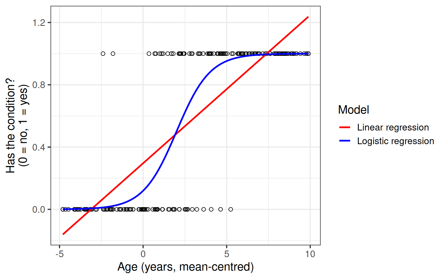
We notice a few things from the plot.
The linear regression model (red line) clearly extends beyond the possible range of values for a probability, which must be between 0 and 1. We can notice negative predictions for the probability associated to low ages, and even predicted probabilities greater than 1 for larger ages. This doesn’t make any sense!
It seems that higher ages are associated with more occurrences of the condition. Similarly, with lower ages we have less occurrences of the condition.
There must be an area in the middle where the probability of having the condition increases sharply, and then the probability is pretty stable in the two ends.
The logistic regression model (blue curve) captures this pattern. In the low ages, the probability of having the condition is very low. For high ages, the probability of having the condition is high (there are barely any people without the condition for mean-centred ages > 5).
There clearly is a zone (ages 0-5) where people have or don’t have the condition. This is where the transition from low to high probability of success occurs.
These exercises will show you how to fit a logistic regression model, and explain how to interpret the parameters.
Introducing GLM
Research Questions
Is susceptibility to change blindness influenced by level of alcohol intoxication and perceptual load?
You may well have already heard of these series of experiments, or have seen similar things on TV.
Question A1
For a given participant in the ‘Door Study,’ give a description of the outcome variable of interest, and ask yourself whether it is binary.
Solution
The outcome variable here is “Did the participant notice the person-swap?”
The values of this are either “Yes” or “No” - they either do or don’t notice that the person they are talking to suddenly changes.
Be careful: The video doesn’t actually state how they are measuring this - via post-experiment question of “did you notice?” or via what the experimenter perceives to be behaviour which indicates awareness of the swap. Always think about what exactly you are measuring.
drunkdoor.csv Dataset
Method
Researchers conducted a study in which they approached 120 people, recruited from within the vicinity of a number of establishments with licenses to sell alcohol to be consumed on-premises. Initially, experimenter A approached participants and asked if they were interested in participating in a short study, and obtained their written consent. While experimenter A subsequently talked each participant through a set of questions on multiple pieces of paper (with the pretense of explaining what the participant was required to do), experimenters B and C carrying a door passed between the participant and experimenter A, with experimenter C replacing A (as can be viewed in the video).
The perceptual load of the experiment was manipulated via a) the presentation of the door and b) the papers held by the experimenters. For 60 of these participants, the door was painted with some detailed graffiti and had a variety of pieces of paper and notices attached to the side facing the participants. Additionally, for these participants, the experimenters handled a disorganised pile of 30 papers, with the top pages covered in drawings around the printed text. For the remaining 60, the door was a standard MDF construction painted a neutral grey, and the experimenters handled only 2 sheets of paper which had minimal printed text on them and nothing else.
Measures
After experimenters A and C had successfully swapped positions, the participant was asked (now by C) to complete small number of questions taking approximately 1 minute. Either after this set of questions, or if the participant made an indication that they had noticed the swap, the experimenters regrouped and the participant was explicitly asked whether they had noticed the swap.
Immediately after this, participants were breathalysed, and their blood alcohol content was recorded.
Blood Alcohol Content (BAC), A BAC of 0.0 is sober, while in the United States 0.08 is legally intoxicated, and above that is very impaired. BAC levels above 0.40 are potentially fatal.
age
Age (in years)
condition
Condition - Perceptual load created by distracting oject (door) and details and amount of papers handled in front of participant (Low vs High)
notice
Whether or not the participant noticed the swap (Yes = 1 vs No = 0)
Question A2
Read in the data, and plot the relationship between the age variable and the notice variable.
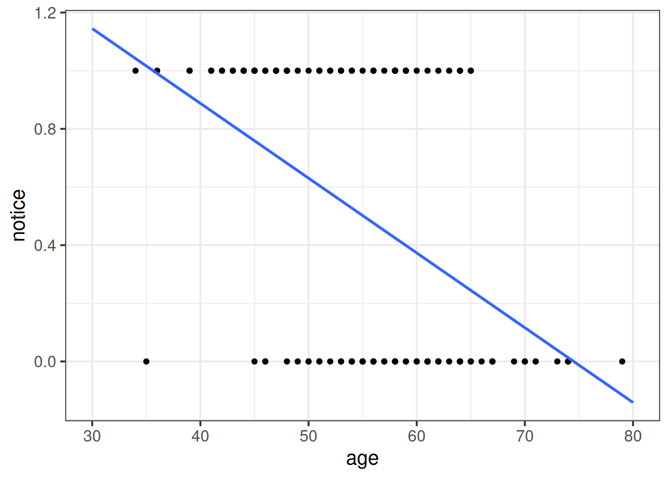
In ggplot, make sure you use geom_point(). Then, add to the plot the following code, geom_smooth(method = "lm", se = FALSE). This will plot a simple linear regression fit lm(notice ~ age).
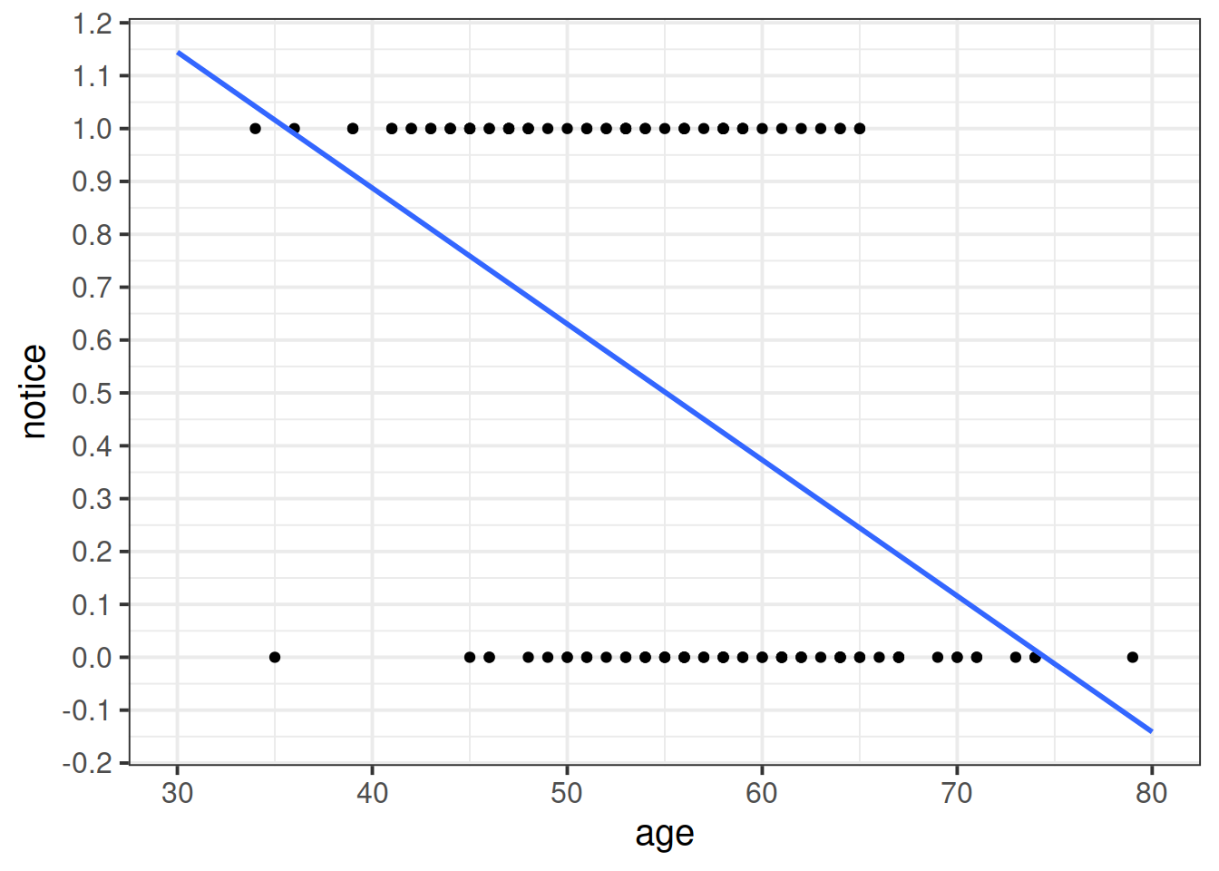
Plot whether or not the swap was noticed vs the age. Also add a simple linear model fit, and we use the fullrange = TRUE argument so that the line spans the entire plot (rather than just the range of the data):
Just visually following the line from the plot produced in the previous question, what do you think the predicted model value would be for someone who is aged 30?
What does this value mean?
Solution
This plot will make it easier to see that the model predicted value for someone aged 30 is approximately 1.15.
But what does 1.15 really mean here? Does it mean that the 30 year old participant will notice 1.15 experimenter-swaps? That doesn’t make sense, there is only one swap. Does it mean that they have a 115% probability of noticing the swap? That is closer, but again it doesn’t make much sense - how can we have a 115% probability?
What we are really interested in here is looking at how specific factors influence the probability of noticing the experimenter-swap.
We also recall that:
a probability must be greater than or equal 0
a probability cannot be larger than 1
Recall that in linear regression we have a term of the following form on the right-hand side of the equal sign
\[
\beta_0 + \beta_1 x_{i1} + \dots + \beta_k x_{ik}
\]
Such term is called a linear predictor because is a linear combination of the predictors.
The possible values of the linear predictor range from \(-\infty\) to \(\infty\). On the contrary, a probability ranges from 0 to 1.
Clearly, we cannot directly model the probability of success as the linear predictor. We need to first transform the probability to range from \(-\infty\) to \(\infty\) and then it is this transformation of the probability that is related to the linear predictor.
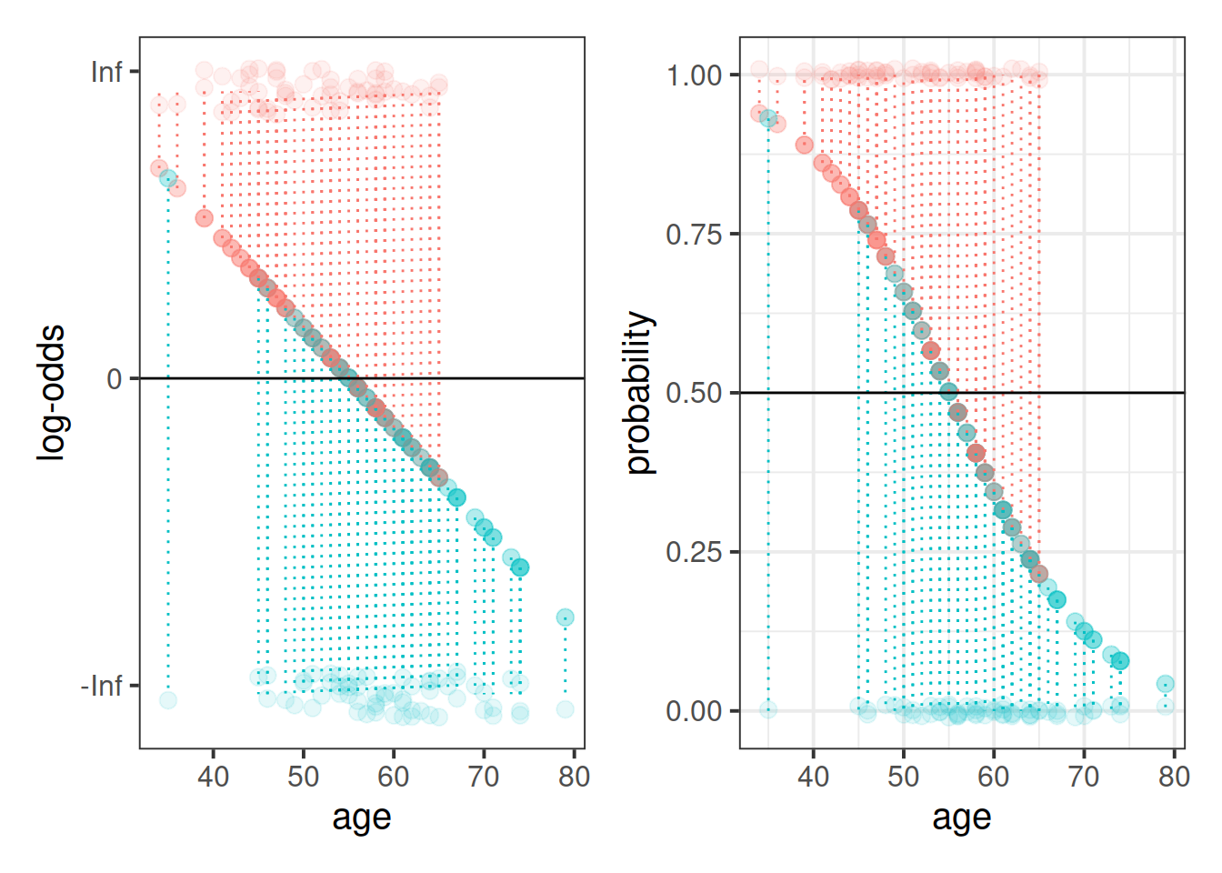
This is where the Generalised Linear Model (GLM) comes in. With a little bit of trickery, we can translate probability (restricted to between 0 and 1, and not represented by a straight line), into “log-odds,” which is both linear and unbounded (see Figure 1).
Probability, odds, log-odds
If we let \(p\) denote the probability of a given event, then:
The probability\(p\) ranges from 0 to 1.
The odds\(\frac{p}{1-p}\) ranges from 0 to \(\infty\).
To see this, consider what happens in the extremes.
The log-odds\(\log \left( \frac{p}{1-p} \right)\) ranges from \(-\infty\) to \(\infty\).
To see this, consider again what happens in the extremes.
When \(\frac{p}{1-p} = 0\), we have \(\log(0) = -\infty\).
When \(\frac{p}{1-p} = \infty\) we have \(\log(\infty) = \infty\).
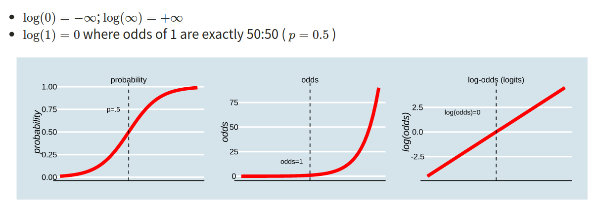
Figure 1: Probability, Odds and Log-odds
Question A4
The probability of a coin landing on heads if 0.5, or 50%. What are the odds, and what are the log-odds?
The 2020 Tour de France winner, Tadej Pogacar, was given odds of 11 to 4 by a popular gambling site (i.e., if we could run the race over and over again, for every 4 he won he would lose 11). Translate this into the implied probability of him winning.
Solution
A 50% chance of landing on heads is equivalent to the odds of \(\frac{0.5}{1-0.5} = \frac{0.5}{0.5} = \frac{1}{1}\) (odds of 1 to 1, i.e., “equal odds”).
The log-odds can be calculated using log(1) in R, which returns 0.
If Pogacar is predicted to win 4 for every 11 he loses, then this is means he is predicted to win 4 in every 15 races, so the implied probability of him winning is \(\frac{4}{15}\) = 0.267.
How is this useful?
Recall the linear model formula we have seen a lot of over DAPR2 so far.
For simplicity, focus on a single predictor \(x_{i1}\) but this can be easily generalised to the case of \(k\) predictors \(x_{i1}, ..., x_{ik}\).
Because we are defining a linear relationship here, we can’t directly model the probabilities (because they are bounded by 0 and 1, and they are not linear). But we can model the log-odds of the event happening.
The logistic regression model requires two components:
One linking the transformed probability (log-odds) to the linear predictor:
\[
\color{red}{\log \left(\frac{p_i}{1-p_i} \right)}
= \color{blue}{\beta_0 + \beta_1 \ x_{i1} }
\]
The second liking the response variable with the probability:
\[
Y_i \sim \text{Binomial}(n, p_i)
\]
For binary responses, \(n = 1\).
The following plot displays the effect of varying the intercept and slope (specified respectively as \((a,b)\)) on the predicted probability of success.
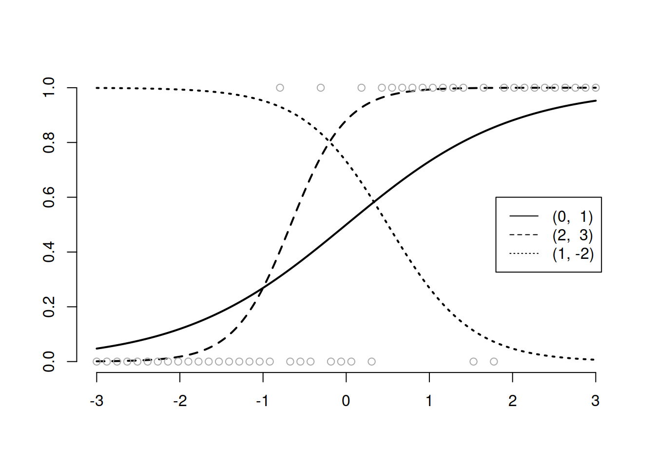
In the above plot it seems like the best curve to fit the probability of success is the one obtained with \(\beta_0 = 2\) and \(\beta_1 = 3\) (dashed line). The dotted line is the worst fit as it gives a high probability of success in an area of no observed success and a low probability of success in an area of high observed successes.
A bit of a tangent - How does the model get estimated?
Maximum Likelihood Estimation
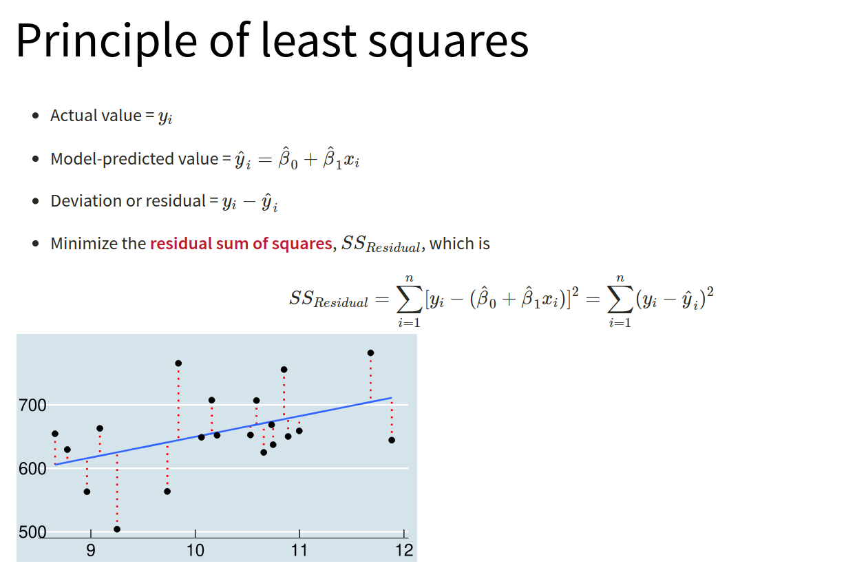
For a linear regression, we heard about how the regression line can be found by “minimising the residual sums of squares” (i.e., we rotate the line to find the point at which \(\sum{(y - \hat{y})^2}\) is smallest. This gave us the “best fitting line” (Figure 2).
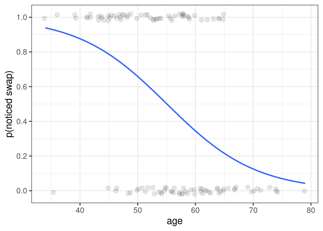
For the logistic regression model, what we’re really wanting is the “best fitting squiggle” (Figure 3), and to get to this we must do something else.
Figure 3: The sigmoid curve
The reason we have to do something different is because for our actual observations, the event has either happened or it hasn’t. So we can’t take the raw data as “probabilities” which we can translate into log-odds. We can try, but it doesn’t make sense, and we would just be trying to fit some line between infinity and negative infinity. This would mean the residuals would also all be infinity, and so it becomes impossible to work out anything!
Instead, maximum likelihood estimation is used to find the set of coefficients which best reproduce the observed data.
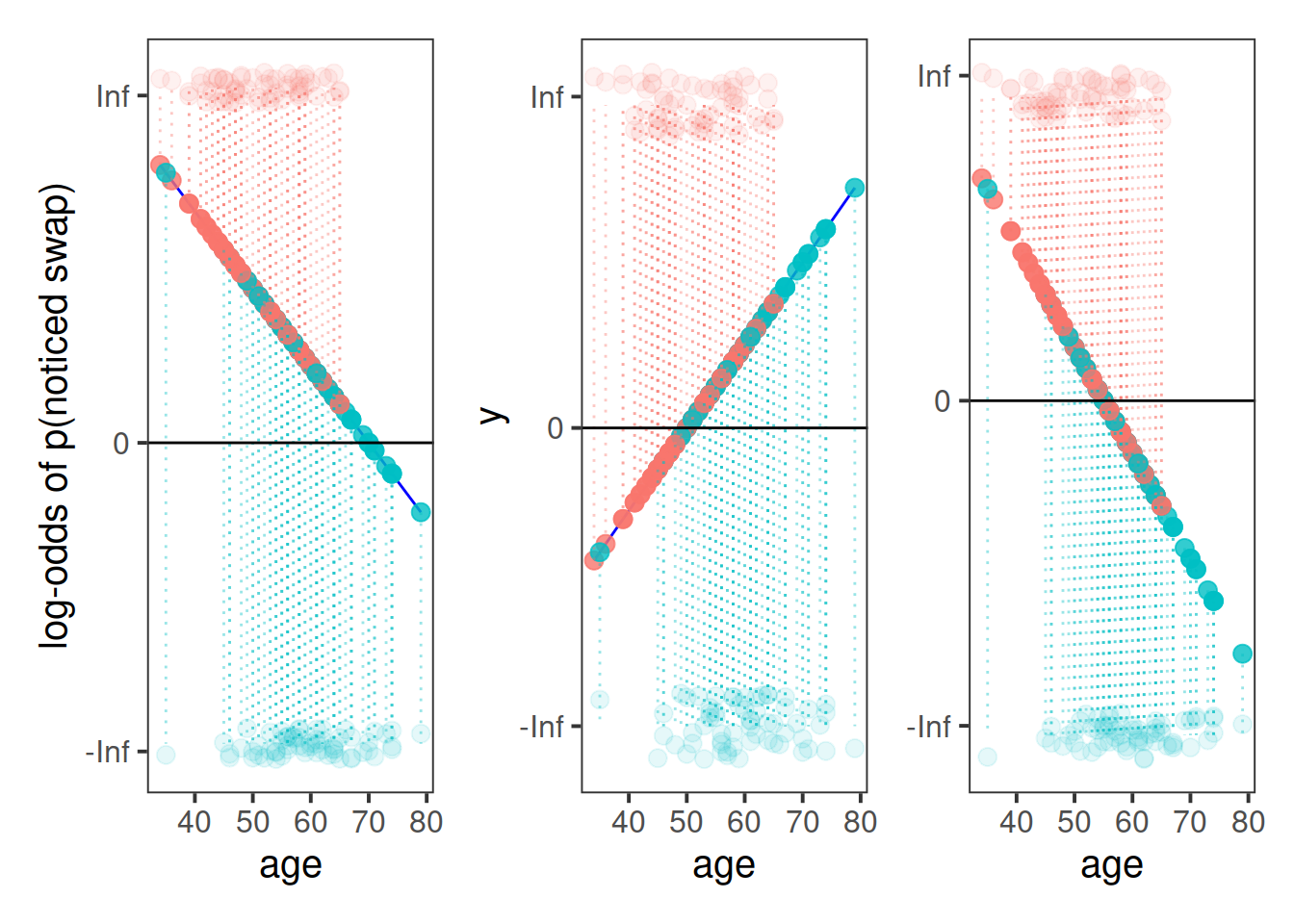
For a given line on the plot where y = log-odds, and x = predictor variable, we can project our points on to it to find some candidate log-odd values for each observation, which we can then compare to the observed data (the 0s and 1s, or -Inf and Inf on the log-odds scale).
Consider three possible lines we might fit below. You can see the observations at the Inf and -Inf points of the y-axis, and they are coloured by whether the event was observed or not. These are then projected down on to the possible lines. Recall that a log-odds of 0 is 50/50, or an odds of 1.
In the left hand plot, all of the observations where the event was observed to happen (red dots at log-odds of +Inf), are modelled as having a log-odds of > 0 (red dots on the line). However, so are a lot of the observations where the event was not observed (blue dots at log-odds of -Inf).
In the middle plot, some red dots get incorrectly given log-odds < 0, and a lot of blue dots get incorrectly given log-odds > 0.
The right hand plot seems to fit a little better - there are only a few points which get given log-odds the wrong way from what we would expect.
Figure 4: Note: the dotted lines are not residuals, but just to show the projections of observations down to the line
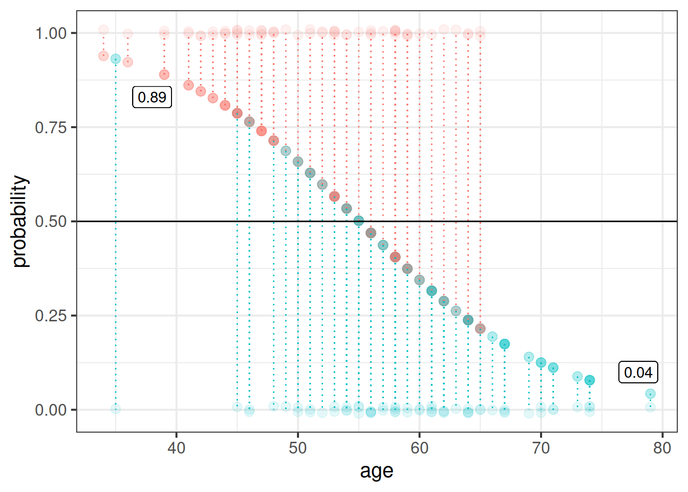
If we take that right-hand plot above, and translate the log-odds back into probabilities, we see the squiggle!
What we can then ask for each of our candidate lines “what is the likelihood of the data, given this line?” To get this, we sum up the probabilities that observed 1s are predicted as 1s and that observed 0s predicted as 0s, at some given threshold which defines what we count as “predicted as 1” (e.g., is the predicted prob < or > 0.5?).
For instance, the furthest right point is an observed 0, and so the likelihood of this data given the predicted probability is 1-0.04, or 0.96.
The cool thing is that computers do all this for us. Maximum likelihood estimation is just a method to find out which parameters maximise the likelihood of the data. In our context, it tells us what values of coefficients in \(\color{red}{\log \left(\frac{p_i}{1-p_i} \right)} = \color{blue}{\beta_0 + \beta_1 x_{i1} }\) maximise the likelihood of reproducing the data we observed.
Question A5
To fit a logistic regression model, we need to useglm(), a slightly more general form of lm().
The syntax is pretty much the same, but we need to add in a family at the end, to tell it that we are doing a binomial logistic regression.
(Note, we’ve been calling our outcome variable “binary,” but now we use “binomial?” Why? Well in the situation that we have a binary outcome consisting of 2 categories represented by 1s and 0s, we actually have a special case of a binomial (“the number of successes in n trials”) where \(n=1\), which is why it often gets referred to as ‘binary logistic regression’)
Using the drunkdoor.csv data, fit a model investigating whether participants’ age predicts the log-odds of noticing the person they are talking to be switched out mid-conversation. Look at the summary() output of your model.
lm(y ~ x1 + x2, data = data)
is the same as:
glm(y ~ x1 + x2, data = data, family = "gaussian")
(Gaussian is another name for the normal distribution)
Solution
model1 <- glm(notice ~ age, data = drunkdoor, family="binomial")
summary(model1)
##
## Call:
## glm(formula = notice ~ age, family = "binomial", data = drunkdoor)
##
## Deviance Residuals:
## Min 1Q Median 3Q Max
## -2.3142 -0.9686 -0.3496 0.9635 1.7526
##
## Coefficients:
## Estimate Std. Error z value Pr(>|z|)
## (Intercept) 7.15625 1.57163 4.553 5.28e-06 ***
## age -0.12999 0.02819 -4.612 4.00e-06 ***
## ---
## Signif. codes: 0 '***' 0.001 '**' 0.01 '*' 0.05 '.' 0.1 ' ' 1
##
## (Dispersion parameter for binomial family taken to be 1)
##
## Null deviance: 166.32 on 119 degrees of freedom
## Residual deviance: 136.84 on 118 degrees of freedom
## AIC: 140.84
##
## Number of Fisher Scoring iterations: 4
Question A6
Interpreting coefficients from a logistic regression can be difficult at first.
Recall what we are modelling - we are no longer modelling \(y\), but the log-odds of \(y\).
Based on your model output, complete the following sentence:
“Being 1 year older decreases _________ by 0.13.”
Solution
“Being 1 year older decreases the log-odds of noticing a mid-conversation person switch by 0.13.”
Question A7
Unfortunately, if we talk about increases/decreases in log-odds, it’s not that intuitive.
What we often do is translate this back into odds.
The opposite of the natural logarithm is the exponential (see here for more details if you are interested), and in R these functions are log() and exp():
log(2)
## [1] 0.6931472
exp(log(2))
## [1] 2
log(exp(0.6931472))
## [1] 0.6931472
Exponentiate the coefficients from your model in order to translate them back from log-odds, and provide an interpretation of what the resulting numbers mean.
Solution
exp(coef(model1))
## (Intercept) age
## 1282.0913563 0.8781015
The odds of noticing a mid-conversation person-switch for someone age 0 is 1282:1.
For every year older someone is, the odds of noticing reduces by a factor of 0.88.
Question A8
Based on your answer to the previous question, calculate the odds of noticing the swap for a one year-old (for now, forget about the fact that this experiment wouldn’t work on a 1 year old!)
And what about for a 40 year old?
Can you translate the odds back to probabilities?
Solution
exp(coef(model1))
## (Intercept) age
## 1282.0913563 0.8781015
The odds of noticing a mid-conversation person-switch for someone age 0 is 1282:1.
For every year older someone is, the odds of noticing reduces by a factor of 0.88.
This means that for a one year old, the odds of noticing are \(1282*0.88\), or 1129:1.
The odds for a 40 year old are \(1282*0.88^{40}\), or 7.71:1
And we can always then turn these back into probabilities.
From probabilities to log-odds (or logit): \[
logit_i=\log \left(\frac{p_i}{1-p_i}\right)
\]
From log-odds to probability: \[
p_i=\frac{e^{logit_i}}{(1+e^{logit_i})}
\]
Predicted probability of noticing for a one year old = \(\frac{1129}{1 + 1129} = 0.99\)
Predicted probability of noticing for a 40 year old = \(\frac{7.71}{1 + 7.71} = 0.89\)
Question A9
We can easily get R to extract these predicted probabilities for us.
Calculate the predicted log-odds (probabilities on the logit scale): predict(model, type="link")
Calculate the predicted probabilities: predict(model, type="response")
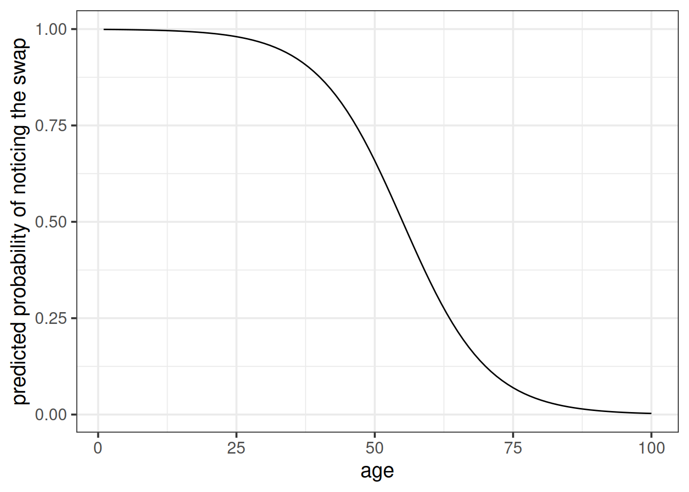
The code below creates a dataframe with the variable age in it, which has the values 1 to 100. Can you use this object in the predict() function, along with your model, to calculate the predicted probabilities of the outcome (noticing the swap) for each value of age? How about then plotting them?
ages100 <- tibble(age = 1:100)
Solution
This will spit out 100 predicted probabilities..
predict(model1, newdata = ages100, type = "response")
ggplot(data = ages100, aes(x = age, y = predprobs)) +
geom_line()+
labs(y="predicted probability of noticing the swap")
Question A9
Shortcut!
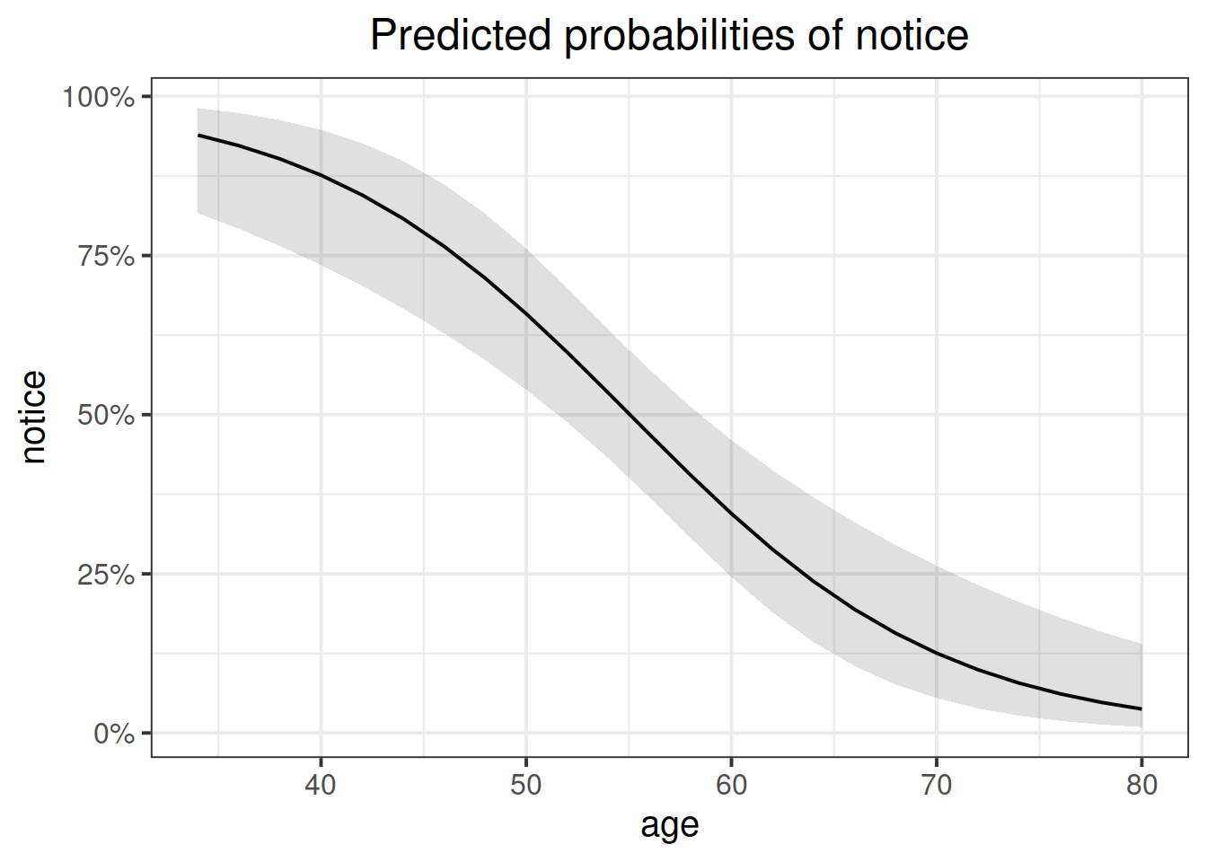
We can do this really easily with the sjPlot package!
Try running this code (replace model1 with the name of your model):
library(sjPlot)
plot_model(model1, type="pred")
Solution
library(sjPlot)
plot_model(model1, type="pred")
## $age
Question A10
We have the following model coefficients, in terms of log-odds:
summary(model1)$coefficients
## Estimate Std. Error z value Pr(>|z|)
## (Intercept) 7.1562479 1.57163317 4.553383 5.279002e-06
## age -0.1299931 0.02818848 -4.611569 3.996402e-06
We can convert these to odds by using exp():
exp(coef(model1))
## (Intercept) age
## 1282.0913563 0.8781015
In order to say something along the lines of “For every year older someone is, the odds of noticing the mid-conversation swap (the outcome event happening) reduces by a factor of 0.88.”
Why can we not translate this into a straightforward statement about the change in probability of the outcome for every year older someone is?
Solution
We have to be careful - we are talking about an odds ratio.
Our model holds that a 21 year old has 0.88 the odds that a 20 year old has, and that a 51 year old has 0.88 the odds of a 50 year old.
But these are not the same in terms of probability. The probability between age and the probability isn’t linear, it is sigmoidal.
example <- tibble(
age = c(20,21,50,51)
)
example <-
example %>% mutate(
logodds = predict(model1, newdata = example, type = "link"),
odds = exp(logodds),
probs = predict(model1, newdata = example, type = "response"),
)
example
This is the same thing we saw visually in Figure 1!
GLM as a classifier
Question B1
From the model we created in the earlier exercises:
model1 <- glm(notice ~ age, data = drunkdoor, family="binomial")
Add new column to the drunkdoor dataset which contains the predicted probability of the outcome for each observation.
Then, using ifelse(), add another column which is these predicted probabilities translated into the predicted binary outcome (0 or 1) based on whether the probability is greater than >.5.
Create a two-way contingency table of the predicted outcome and the observed outcome.
Hint: you don’t need the newdata argument for predict() if you want to use the original data the model was fitted on.
A table of predicted outcome vs observed outcome sometimes gets referred to as a confusion matrix, and we can think of the different cells in general terms (Figure 5).
Another way to think about how our model is fitted is that it aims to maximise (TP + TN)/n, or, put another way, to minimise (FP+FN)/n.
Which is equivalent to the good old idea of minimising sums of squares (where we minimise the extend to which the predicted values differ from the observed values).
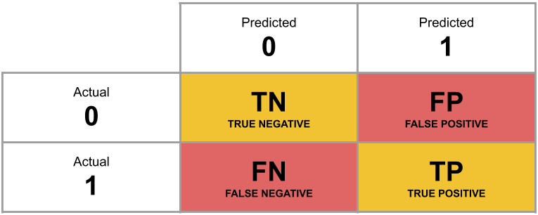
Figure 5: Confusion Matrix
Question B2
What percentage of the n = 120 observations are correctly classified by our model, when the threshold is set at 0.5?
The model correctly classifies 67.5% of the observations.
Less guided exercises
Approaching a research question
Question C1
Recall our research question, which we will now turn to:
Research Questions
Is susceptibility to change blindness influenced by level of alcohol intoxication and perceptual load?
Try and make a mental list of the different relationships between variables that this question invokes, can you identify one variable as the ‘outcome’ or ‘response’ variable? (it often helps to think about the implicit direction of the relationship in the question)
Solution
The question seems to ask about two relationships:
susceptibility to change blindness ← alcohol intoxication
susceptibility to change blindness ← perceptual load
The arrows above are used to show the implied direction of the influence, and in the lm()/glm() syntax, you could imagine each of these mapping to a formula syntax we have seen a few times (e.g., t.test(data$outcome ~ data$group) and lm(outcome ~ predictor)). We can see that the ‘susceptibility to change blindness’ is our outcome variable:
change blindness ~ alcohol
change blindness ~ perceptual load
As a general rule of thumb, it is often worth asking yourself “why run two models when one will do?” Think about what we have learned about moving from simple to multiple regression - some of the explanatory power of x in the relationship y~x might be shared by the relationship y~z.
This will depend on precisely what quantity you want to estimate, i.e., “the overall effect of \(x\) on \(y\)independent of \(z\)” or “the effect of \(x\) on \(y\)after partialling out the effect of \(z\) on \(y\).” The former statement might indicate a simple bivariate relationship, and the latter requires more advanced techniques (e.g., multiple regression).
Question C2
Think about our outcome variable and how it is measured. What type of data is it? Numeric? Categorical?
What type of distribution does it follow? For instance, do values vary around a central point, or fall into one of various categories, or follow the count of successes in a number of trials?
Solution
Our outcome variable here is drunkdoor$notice, and is stored as a set of 0s and 1s. These are the only two values that an observation can take, and they represent the number of successes in \(n = 1\) trials.
So, from this we learn that our method of analysis should be suited to model this binary outcome. So things like lm() and t.test() are not very appropriate.
Question C3
Think about our explanatory variable(s). Is there more than one? What type of variables are they? Do we want to model these together? Might they be correlated?
Are there any other variables (measured or unmeasured) which our prior knowledge or theory suggests might be relevant?
Solution
We know that drunkdoor$bac is simply the observed blood alcohol level (BAC). This is technically measured as a proportion, but for the current purposes we can just treat it as any other numeric scale. However, we might consider scaling the variable so that instead of the coefficient representing the change when moving from 0% to 1% BAC (1% blood alcohol is fatal!), we might want to have the change associated with 0% to 0.01% BAC (i.e, a we want to talk about effects in terms of changing 1/100th of a percentage of BAC).
The drunkdoor$condition variable is an experimental manipulation. That is, the researchers had control over what observations fell into which group. We wouldn’t therefore expect any correlation between this and the bac variable (unless researchers did not allocate participants to conditions randomly).
If we were actually doing research in this area, we might already have the idea based on previous research that change-blindness appears to vary depending upon age. From the earlier exercises here we have some evidence to corroborate this. We may therefore want to include this in our model. If we don’t, any results might simply be due to, e.g. older people tending to be more highly intoxicated (and so we see an effects of alcohol that might actually be simply the effect of age).
We might also think about any other possible variables which might influence our results, even if we didn’t measure them. This sort of thinking becomes important in the discussion section.
John Stuart Mill - Three Criteria for Causality
To varying extents, all of these criteria can be incredibly difficult to satisfy. Criteria 3 especially is one of the things that makes scientific investigation so interesting.
The cause precedes the effect
The cause is demonstrably related to the effect
There are no plausible alternative explanations
Mill, J. S. (1869). A System of Logic, Ratiocinative and Inductive: Being a Connected View of the Principles of Evidence and the Methods of Scientific Investigation. Harper and brothers.
Fitting the model
Question C4
Write a sentence describing the model you will fit. It might help to also describe each variable as you introduce it.
Fit the model.
Things to think about:
Do you want BAC on the current scale, or could you transform it somehow?
Is condition a factor? What is your reference level? Have you checked contrasts(drunkdoor$condition)? (This will only work if you make it a factor first)
Solution
Whether or not participants noticed the swap mid-conversation (binary 0 vs 1) was modelled using logistic regression, with blood alcohol content (measured in 100th of percentages blood content) and perceptual load condition (low load vs high load, with low as the reference level) and age (years).
In the sentence above, I stated that I want blood alcohol in terms of 100ths of percentages, rather than percentages.
I also stated that the low-load will be the reference level.
Currently it is the other way around:
# make it a factor
drunkdoor$condition<-factor(drunkdoor$condition)
contrasts(drunkdoor$condition)
## Low
## High 0
## Low 1
So let’s change it:
# change 0,1 column to 1,0, and rename it so it
# compares high against low (not low against high)
contrasts(drunkdoor$condition) <- cbind(High=c(1,0))
contrasts(drunkdoor$condition)
## High
## High 1
## Low 0
changeblind_model <- glm(notice ~ bac100 + condition + age, data = drunkdoor, family = "binomial")
summary(changeblind_model)
##
## Call:
## glm(formula = notice ~ bac100 + condition + age, family = "binomial",
## data = drunkdoor)
##
## Deviance Residuals:
## Min 1Q Median 3Q Max
## -2.01149 -0.31516 -0.00735 0.26706 2.23101
##
## Coefficients:
## Estimate Std. Error z value Pr(>|z|)
## (Intercept) 17.01764 3.55483 4.787 1.69e-06 ***
## bac100 0.60763 0.17431 3.486 0.000491 ***
## conditionHigh -5.60871 1.11634 -5.024 5.06e-07 ***
## age -0.30482 0.06232 -4.891 1.00e-06 ***
## ---
## Signif. codes: 0 '***' 0.001 '**' 0.01 '*' 0.05 '.' 0.1 ' ' 1
##
## (Dispersion parameter for binomial family taken to be 1)
##
## Null deviance: 166.322 on 119 degrees of freedom
## Residual deviance: 66.763 on 116 degrees of freedom
## AIC: 74.763
##
## Number of Fisher Scoring iterations: 6
Question C5
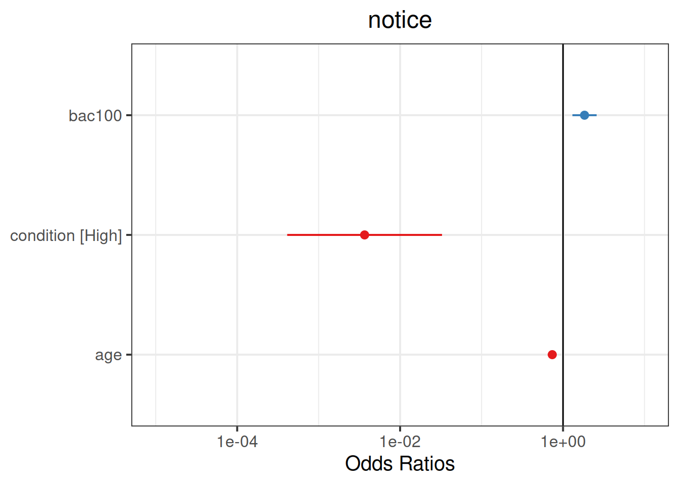
Compute 95% confidence intervals for the log-odds coefficients using confint(). Wrap the whole thing in exp() in order to convert all these back into odds and odds-ratios.
Try the sjPlot package and using plot_model() on your model, but with type="est". What do you get?
Tip:, for some people this plots seems to miss out plotting the BAC effect, so you might need to add:
sjPlot::plot_model(changeblind_model, type = "est")+
geom_hline(yintercept=1)+
scale_y_log10(limits = c(1e-05,10))
Looking beyond
This week we have looked at one specific type of Generalised Linear Model, in order to fit a binary logistic regression. We can use GLM to fit all sorts of models, depending on what type of data our outcome variable is, and this is all through the family = part of the model syntax.
For instance, if we had data which was binomial but with an \(n > 1\), for instance the number of correct answers in 10 trials:
participant
trials_correct
trials_incorrect
x1
id1
1
9
114
id2
4
6
113
id3
7
3
83
id4
8
2
141
id5
3
7
115
...
...
...
...
We could model this with family = "binomial" using the two columns as the outcome: glm(cbind(trials_correct, trials_incorrect) ~ x1, data = data, family = "binomial")
Or if we had count data, which can range from 0 to Infinity (theoretically), e.g.:
person
n_fish_caught
age
id1
8
44
id2
7
46
id3
13
29
id4
6
56
id5
14
37
...
...
...
We model this using family = "poisson": glm(n_fish_caught ~ age, data = data, family = "poisson")
For real studies demonstrating the effects used in the example here, see:
A note: This sort of binary thinking can be useful, but it is important to remember that it can in part be simply a result of measurement. To answer some research questions, we need to consider an event as “success” = 1 and all other possibilities as “failure” = 0.
For instance, we might initially consider “has blond hair” to be binary “Yes/No,” but that doesn’t mean that in the real world people either have blond hair or they don’t. We could instead choose to measure hair colour via colorimetric measures of the energy at each spectral wavelength, meaning “blondness” could become a continuum. While binary thinking can be useful, it is not difficult to think of ways in which it can be harmful.↩︎