Writing-up

Be sure to check the solutions to last week’s exercises.
You can still ask any questions about previous weeks’ materials if things aren’t clear!

LEARNING OBJECTIVES

1. Understand the difference between outliers and influential points.
2. Understand and apply methods to detect outliers and influential points.
3. Comment on the issues of correlation vs causation and generalisability of the sample results.
4. Run a full simple regression analysis from start to finish and to correctly interpret the results.

Research question

A group of researchers is interested in the relationship between the reaction time taken by people to identify whether two 3D images display the same object or not, and the rotation angle at which one of the two objects is presented.

Consider the following data containing the reaction times (in milliseconds) it took a sample of 100 people to identify whether two 3D objects were the same or not, for different rotation angles between 0 and 200 degrees.

Data: mental_rotation.csv. Click the plus to expand →

Download link

Download the data here

Description

Each person in the sample was asked to look at two 3D images presented next to each other. The second image was simply a rotated version of the first, and the participants were asked to identify if the two images showed the same object or not. The reaction time (in milliseconds) was recorded for each participant.

The measured variables were:

• angle_degrees: The rotation angle, between 0 and 200 degrees, of the second image.
• rt_ms: Reaction time (in milliseconds).

Figure 1: Example of target object (left) and rotated version of it (right). Source: https://plato.stanford.edu/entries/mental-imagery/mental-rotation.html

Preview

The first six rows of the data are:

angle_degrees	rt_ms
69.23	882.99
3.08	541.60
164.62	1618.78
153.85	1458.74
63.08	973.34
21.54	627.80

Analysis

IMPORTANT

In today’s lab the analysis is provided, and the task for you will be to correctly report what has been done and why.

Read the data into R:

library(tidyverse)
library(car)

mr <- read_csv(file = 'https://uoepsy.github.io/data/mental_rotation.csv')
head(mr)

## # A tibble: 6 x 2
##   angle_degrees rt_ms
##           <dbl> <dbl>
## 1         69.2   883.
## 2          3.08  542.
## 3        165.   1619.
## 4        154.   1459.
## 5         63.1   973.
## 6         21.5   628.

Rename variables:

mr <- mr %>%
  rename(
    angle = angle_degrees,
    rt = rt_ms
  )
head(mr)

## # A tibble: 6 x 2
##    angle    rt
##    <dbl> <dbl>
## 1  69.2   883.
## 2   3.08  542.
## 3 165.   1619.
## 4 154.   1459.
## 5  63.1   973.
## 6  21.5   628.

TIP

The patchwork library is used to combine ggplots into a single figure made up of multiple panels. You can add individual ggplots using + or |, and put plots underneath with the / operator.

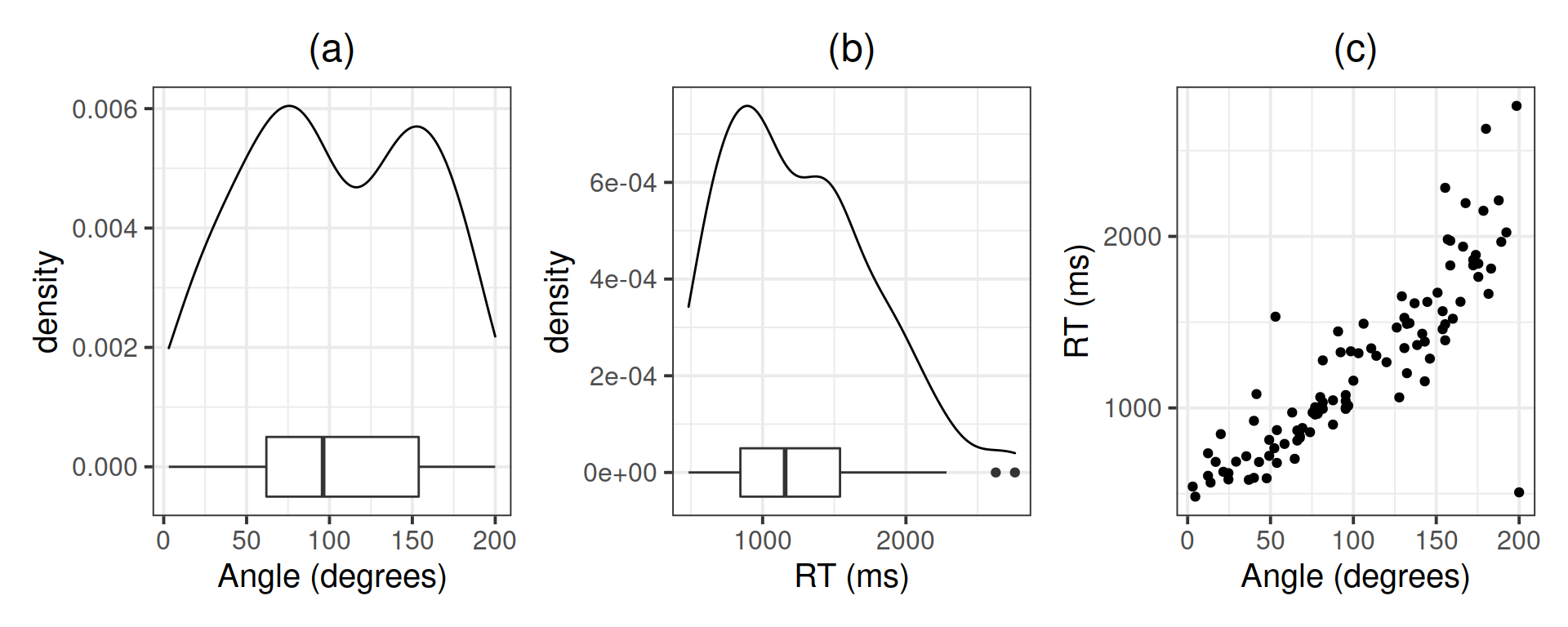
Investigate the marginal distribution of each variable and the relationship between the two variables.

library(patchwork)

plt_angle <- ggplot(mr, aes(x = angle)) +
  geom_density() +
  geom_boxplot(width = 0.001) +
  labs(x = 'Angle (degrees)')

plt_rt <- ggplot(mr, aes(x = rt)) +
  geom_density() +
  geom_boxplot(width = 0.0001) +
  labs(x = 'RT (ms)')

plt_joint <- ggplot(mr, aes(x = angle, y = rt)) +
  geom_point() +
  labs(x = 'Angle (degrees)', y = 'RT (ms)')

plt_angle | plt_rt | plt_joint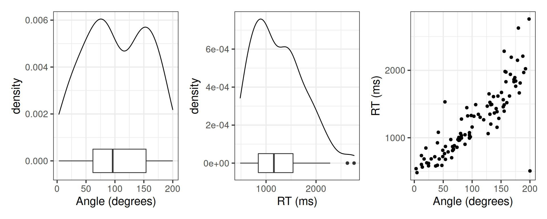

mr %>%
  summarise(M_angle = mean(angle), 
            SD_angle = sd(angle),
            MED_angle = median(angle), 
            IQR_angle = IQR(angle),
            M_rt = mean(rt), 
            SD_rt = sd(rt),
            MED_rt = median(rt), 
            IQR_rt = IQR(rt))

## # A tibble: 1 x 8
##   M_angle SD_angle MED_angle IQR_angle  M_rt SD_rt MED_rt IQR_rt
##     <dbl>    <dbl>     <dbl>     <dbl> <dbl> <dbl>  <dbl>  <dbl>
## 1    103.     54.3      96.2      91.9 1243.  505.  1157.   695.

Correlation between the variables:

cor(mr)

##           angle        rt
## angle 1.0000000 0.8540206
## rt    0.8540206 1.0000000

Linear model:

mdl1 <- lm(rt ~ 1 + angle, data = mr)
summary(mdl1)

## 
## Call:
## lm(formula = rt ~ 1 + angle, data = mr)
## 
## Residuals:
##      Min       1Q   Median       3Q      Max 
## -1503.24  -126.76   -26.26    84.89   774.49 
## 
## Coefficients:
##             Estimate Std. Error t value Pr(>|t|)    
## (Intercept) 422.9043    56.9626   7.424  4.2e-11 ***
## angle         7.9417     0.4887  16.251  < 2e-16 ***
## ---
## Signif. codes:  0 '***' 0.001 '**' 0.01 '*' 0.05 '.' 0.1 ' ' 1
## 
## Residual standard error: 264 on 98 degrees of freedom
## Multiple R-squared:  0.7294, Adjusted R-squared:  0.7266 
## F-statistic: 264.1 on 1 and 98 DF,  p-value: < 2.2e-16

TIP

When you call plot() on a fitted model to show the diagnostic plots, you can display all four plots at once by telling R:

par(mfrow = c(2,2))

This means that each figure should be made of 2 by 2 plots, filled row-wise. The first plot will appear in panel (1,1), the second plot in panel (1,2), the third in panel (2,1) and the last in panel (2,2).

To go back to one figure made of a single plot, you type:

par(mfrow = c(1,1))

IMPORTANT

par(mfrow = ...) will not work with ggplot.

Diagnostics:

par(mfrow = c(2,2))
plot(mdl1)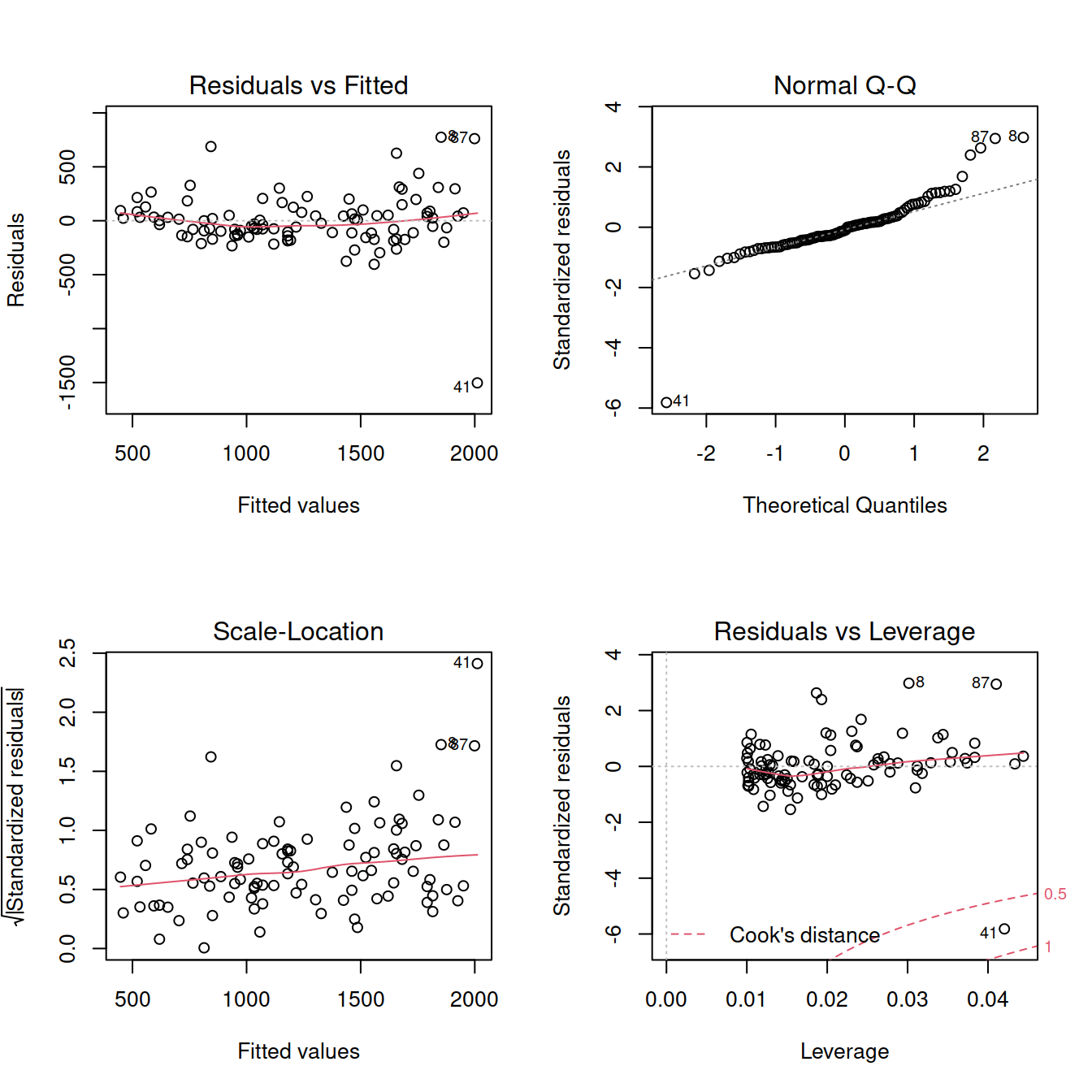

im <- influence.measures(mdl1)
summary(im)

## Potentially influential observations of
##   lm(formula = rt ~ 1 + angle, data = mr) :
## 
##    dfb.1_ dfb.angl dffit   cov.r   cook.d  hat  
## 2   0.08  -0.07     0.08    1.07_*  0.00    0.04
## 8  -0.25   0.45     0.55_*  0.87_*  0.14    0.03
## 19 -0.10   0.24     0.34    0.92_*  0.06    0.02
## 41  0.82  -1.31_*  -1.50_*  0.46_*  0.74_*  0.04
## 52  0.02  -0.02     0.02    1.07_*  0.00    0.04
## 63  0.35  -0.26     0.37    0.90_*  0.07    0.02
## 87 -0.34   0.55     0.63_*  0.88_*  0.19    0.04

For now, we will focus on Cook’s distance only:

mr <- mr[-41, ]

Re-fit the model using the new dataset and check the assumptions:

mdl2 <- lm(rt ~ 1 + angle, data = mr)
summary(mdl2)

## 
## Call:
## lm(formula = rt ~ 1 + angle, data = mr)
## 
## Residuals:
##     Min      1Q  Median      3Q     Max 
## -440.29 -132.78  -27.69   64.74  718.91 
## 
## Coefficients:
##             Estimate Std. Error t value Pr(>|t|)    
## (Intercept)  384.897     46.632   8.254 7.72e-13 ***
## angle          8.462      0.404  20.942  < 2e-16 ***
## ---
## Signif. codes:  0 '***' 0.001 '**' 0.01 '*' 0.05 '.' 0.1 ' ' 1
## 
## Residual standard error: 214.7 on 97 degrees of freedom
## Multiple R-squared:  0.8189, Adjusted R-squared:  0.817 
## F-statistic: 438.6 on 1 and 97 DF,  p-value: < 2.2e-16

par(mfrow = c(2,2))
plot(mdl2)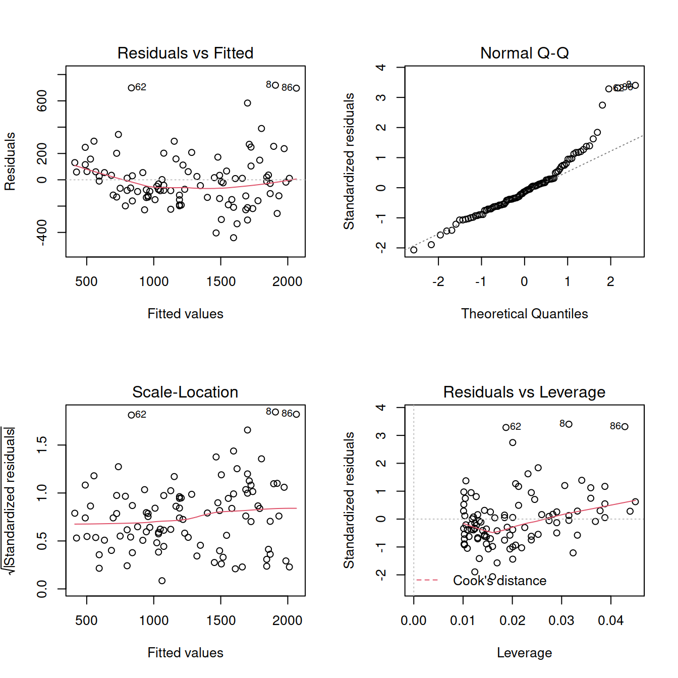

ncvTest(mdl2)

## Non-constant Variance Score Test 
## Variance formula: ~ fitted.values 
## Chisquare = 11.15201, Df = 1, p = 0.00083941

Try transforming the response:

mr <- mr %>%
    mutate(log_rt = log(rt))

Fit a linear model using the transformed response:

mdl3 <- lm(log_rt ~ 1 + angle, data = mr)
summary(mdl3)

## 
## Call:
## lm(formula = log_rt ~ 1 + angle, data = mr)
## 
## Residuals:
##      Min       1Q   Median       3Q      Max 
## -0.28639 -0.09377 -0.01471  0.07431  0.63128 
## 
## Coefficients:
##              Estimate Std. Error t value Pr(>|t|)    
## (Intercept) 6.3291728  0.0330909   191.3   <2e-16 ***
## angle       0.0070543  0.0002867    24.6   <2e-16 ***
## ---
## Signif. codes:  0 '***' 0.001 '**' 0.01 '*' 0.05 '.' 0.1 ' ' 1
## 
## Residual standard error: 0.1524 on 97 degrees of freedom
## Multiple R-squared:  0.8619, Adjusted R-squared:  0.8605 
## F-statistic: 605.3 on 1 and 97 DF,  p-value: < 2.2e-16

par(mfrow = c(2,2))
plot(mdl3)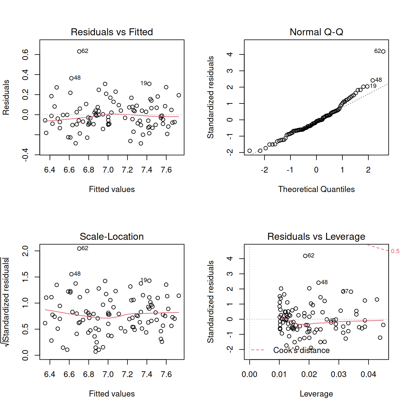

shapiro.test(mdl3$residuals)

## 
##  Shapiro-Wilk normality test
## 
## data:  mdl3$residuals
## W = 0.95174, p-value = 0.001159

Try removing the outlier from the dataset:

mr <- mr[-62, ]

Re-fit the model and check assumptions:

mdl4 <- lm(log_rt ~ 1 + angle, data = mr)
summary(mdl4)

## 
## Call:
## lm(formula = log_rt ~ 1 + angle, data = mr)
## 
## Residuals:
##      Min       1Q   Median       3Q      Max 
## -0.28447 -0.08552 -0.01535  0.07567  0.37662 
## 
## Coefficients:
##              Estimate Std. Error t value Pr(>|t|)    
## (Intercept) 6.3111856  0.0303685  207.82   <2e-16 ***
## angle       0.0071666  0.0002621   27.34   <2e-16 ***
## ---
## Signif. codes:  0 '***' 0.001 '**' 0.01 '*' 0.05 '.' 0.1 ' ' 1
## 
## Residual standard error: 0.1387 on 96 degrees of freedom
## Multiple R-squared:  0.8862, Adjusted R-squared:  0.885 
## F-statistic: 747.8 on 1 and 96 DF,  p-value: < 2.2e-16

par(mfrow = c(2,2))
plot(mdl4)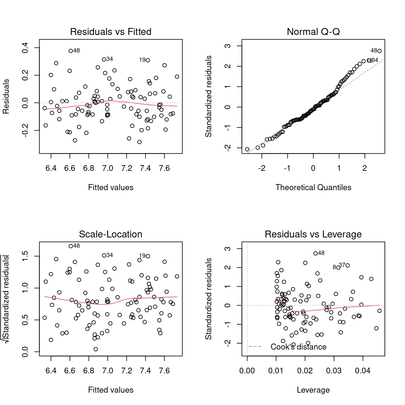

shapiro.test(mdl4$residuals)

## 
##  Shapiro-Wilk normality test
## 
## data:  mdl4$residuals
## W = 0.97986, p-value = 0.138

ncvTest(mdl4)

## Non-constant Variance Score Test 
## Variance formula: ~ fitted.values 
## Chisquare = 0.2260013, Df = 1, p = 0.6345

Go back to figures with only one plot:

par(mfrow = c(1,1))

Create a table for reporting the results:

library(sjPlot)
tab_model(mdl4)

	log rt
Predictors	Estimates	CI	p
(Intercept)	6.31	6.25 – 6.37	<0.001
angle	0.01	0.01 – 0.01	<0.001
Observations	98
R2 / R2 adjusted	0.886 / 0.885

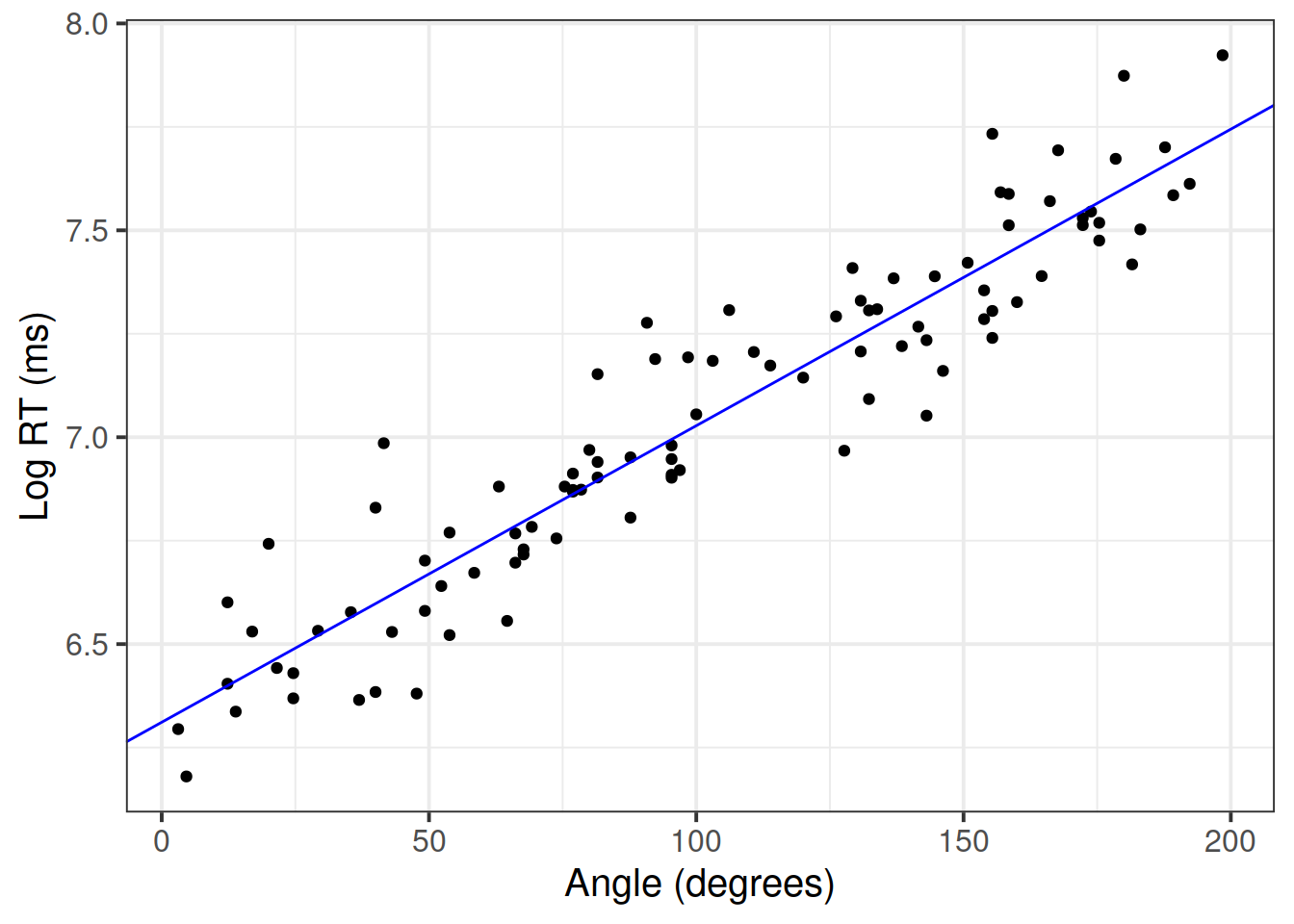
Plot the final model:

betas <- coef(mdl4)

ggplot(mr, aes(x = angle, y = log_rt)) +
  geom_point() +
  geom_abline(intercept = betas[1], slope = betas[2], color = 'blue') +
  labs(x = 'Angle (degrees)', y = 'Log RT (ms)')

Reporting

A good data analysis report should follow three steps: Think, Show, and Tell.

For a detailed explanation of each step, check this document.

Think

What do you know? What do you hope to learn? What did you learn during the exploratory analysis?

1: Describe design

Describe the study design, the data collection strategy, etc.

Solution

A random sample of 100 participants was invited to take part into a mental rotation task. Each participant was shown two images and was asked to identify whether or not the objects displayed in the two images were the same. The second image was displayed with a rotation of a certain angle. For each participant, reaction time (in milliseconds) and rotation angle (in degrees) were recorded.

2: Describe the data

• How many observational units? (If not mentioned above.)
• Are there any observations that have been excluded based on pre-defined criteria? How/why, and how many?
• Describe and visualise the variables of interest. How are they scored? have they been transformed at all?
• Describe and visualise relationships between variables. Report covariances/correlations.

Solution

Figure 2: Marginal and joint distributions.

The distribution of rotation angles appears to be roughly symmetric around the mean angle of 103 degrees, with standard deviation 54.3 degrees. The boxplot in Figure 2(a) does not highlight any evident outliers.

The distribution of reaction times appears to be right skewed, with a median reaction time of 1157 ms, and interquartile range of 695 ms. A boxplot of the distribution, Figure 2(b), flags two potential outliers which are worth keeping an eye on, but have not been removed from the dataset.

Finally, the scatterplot in Figure 2(c) displays the relationship between rotation angle and reaction time. There appears to be a strong (\(r_{Angle, RT} = 0.81\)), positive linear relationship between the two variables. The scatterplot also highlights a couple of points which do not fit with the rest of the data. One has a high rotation angle but an unusually low reaction time, and another point having an angle of approximately 50 degrees and a reaction time of 1500 ms approximately, which is roughly 700 ms above the rest of the points.

3: Describe the analytical approach

• What type of statistical analysis do you use to answer the research question? (e.g., t-test, simple linear regression, multiple linear regression)
• Describe the model/analysis structure
• What is your outcome variable? What is its type?
• What are your predictors? What are their types?
• Any other specifics?

Solution

We want to investigate whether reaction time is affected by the object’s rotation angle and what is the intensity of that relationship.

To do so, we will use a simple linear regression model involving two numeric variables: angle (the predictor) and reaction time (the response). In the dataset, angle is measured in degrees and reaction time in milliseconds.

4: Planned analysis vs actual analysis

• Was there anything you had to do differently than planned during the analysis? Did the modelling highlight issues in your data?
• Did you have to do anything (e.g., transform any variables, exclude any observations) in order to meet assumptions?

Solution

The linear model \(\widehat{RT} = \hat \beta_0 + \hat \beta_1 Angle\), however, highlighted one influential observation (namely, case 41) having a Cook’s distance of 0.74. Careful inspection of case 41 showed a large rotation angle (200 degrees), far from the average angle (103 degrees) — hence, the point has high leverage. Furthermore, the point was an outlier as the actual reaction time was 508 ms, which was roughly 1503 ms lower than the model-predicted value.

After removing such observation from the dataframe and re-fitting the linear model, the diagnostic plots raised concerns about the normality and equal variance assumptions not being satisfied.

The Normal quantile plot showed that the distribution of the residuals was skewed to the right, and the Scale-Location plot displayed a thickening pattern (that is, a fan-shape) rather than a roughly constant vertical spread. Similarly, the Residuals vs Fitted values plot also showed a thickening pattern with a fan-like shape, suggesting a violation of the constant variance assumption.

To mitigate the violation of the equal variance assumption, we log transformed the response variable.

After refitting the model, the diagnostic plots only raised concern about a single point (case 62) not fitting the linear pattern in the Normal quantile plot, and also being particularly unusual in the Residuals vs Fitted values plot.

At the 5% significance level, a Shapiro-Wilk test for normality of the errors showed a significant p-value, indicating violation of the normality assumption.

After careful inspection, we decided to remove case 62 from the dataset and re-fit the linear model.

Show

Show the mechanics and visualisations which will support your conclusions

5: Present and describe the final model

Present and describe the model or test which you deemed best to answer your question.

Solution

The final model which was chosen to answer the research question of interest was: \[ \widehat{\log (RT)} = 6.31 + 0.00717 \ Angle \]

and was fitted excluding case 41, and then case 62.¹ The former was found to be an influential point, while the latter an outlier affecting normality.

6: Are the assumptions and conditions of your final test or model satisfied?

Are the assumptions and conditions of your final test or model satisfied? For the final model (the one you report results from), were all assumptions met? (Hopefully yes, or there is more work to do…). Include evidence (tests or plots).

Solution

The final model was found to not violate the regression assumptions. A plot of the residuals vs fitted values shows randomly scattered points with no pattern and a horizontal direction.

The Normal quantile plot (qq-plot) shows a roughly linear trend in the standardized residuals vs the normal quantiles. We performed a Shapiro-Wilk test, at the 5% significance level, against the null hypothesis that the residuals came from a normal distribution (\(W = 0.98\), \(p = 0.138\)). The large \(W\)-statistic leads to a p-value (0.138) larger than the 0.05 threshold. Hence, the sample results do not provide sufficient evidence to reject the null hypothesis that the errors follow a normal distribution.

The Residuals vs Fitted plot and the Scale-Location plot show that the vertical spread of the residuals is roughly the same everywhere. Hence, we see no violation of the constant variance assumption. At the 5% significance level, we also performed a Breusch-Pagan test against the null hypothesis of homoscedasticity (\(\chi^2(1) = 0.226, p = 0.634\)). The large p-value indicates that the sample results do not provide sufficient evidence to reject the null hypothesis of equal variance.

Finally, a plot of residuals vs leverage does not highlight any influential observations.

7: Report your test or model results

• Provide a table of results if applicable (for regression tables, try tab_model() from the sjPlot package).
• Provide plots if applicable.

Solution

The table below displays the estimated regression coefficients along with the corresponding test of significance:

	log rt
Predictors	Estimates	CI	p
(Intercept)	6.31	6.25 – 6.37	<0.001
angle	0.01	0.01 – 0.01	<0.001
Observations	98
R2 / R2 adjusted	0.886 / 0.885

The fitted model is displayed below:

Tell

Communicate your findings

8: Interpret your results in the context of your research question.

• What do your results suggest about your research question?
• Make direct links from hypotheses to models (which bit is testing hypothesis)
• Be specific - which statistic did you use/what did the statistical test say? Comment on effect sizes.
• Make sure to include measurement units where applicable.

Solution

The fitted model predicts log reaction time for a given rotation angle. Both intercept (\(t(96) = 6.31, p < .001\), two-sided) and slope (\(t(96) = 0.00717, p < .001\), two-sided) are significantly different from zero.

The estimated intercept \(\hat \beta_0 = 6.31\) represents the predicted log reaction time (in milliseconds) when the object is not rotated (zero degrees angle).

The estimated slope, \(\hat \beta_1 = 0.00717\), indicates that, each one-degree increase in the object rotation angle is associated, on average, to a 0.00717 ms increase in log reaction time.

That is, there is a positive/increasing linear relationship between rotation angle and log reaction time. However, the magnitude of the rate of increase, even if significant, is small and in the order of 0.01.

The F-test for model utility is also significant (\(F(1,96) = 747.8, p < .001\)). At the 5% significance level, rotation angle is a significant predictor of log reaction time.²

Approximately 88.6% of the variability in log reaction times is explained by the linear association with the objects’ rotation angle.

Put everything together

If you followed the steps above, it is just a matter of taking all answers to the above questions and combining them, in order to have a reasonable draft of a statistical report.

---

1. Footnote: in the original dataset, these would be cases 41 and 63.↩︎

2. In simple linear regression, this information is equivalent to the t-test for the significance of the slope as the F-statistic is the square t-statistic.↩︎