Getting started with R and RStudio

1 Getting R and RStudio

1.1 Accessing the software

Recommended option: access it via the RStudio server. Try these steps first to register for RStudio server online:

Log in to EASE using your university UUN and password.
Set your RStudio password here, the username will be the same as your UUN (make sure you type your UUN correctly).
Access the server from https://rstudio.ppls.ed.ac.uk using your university UUN and the password you set above in (2).

If the steps above did not work:

Please complete this form and wait for an email. Please note that this can take up to four working days.
Once you receive an email from us, please follow the following instructions:
- Set your here, the username will be the same as your UUN (make sure you type your UUN correctly).
- Access the server from https://rstudio.ppls.ed.ac.uk using your university UUN and the password you just set above.

Alternative: install it locally on your PC following these instructions.

1.2 Setting up your folder

Create a new folder on the server. Give it a useful name like the name of the course: DAPR1. (In the picture we have used “USMR” but please use “DAPR1”).

In the top right, click Project > New Project

Click “Existing Directory”

Click “Browse” and then choose the folder you just created. Click “Choose” and then click “Create Project”.

You should now be able to tell that you have the project open, because it shows you in the top right.

You’re ready to go!

2 A first look at RStudio

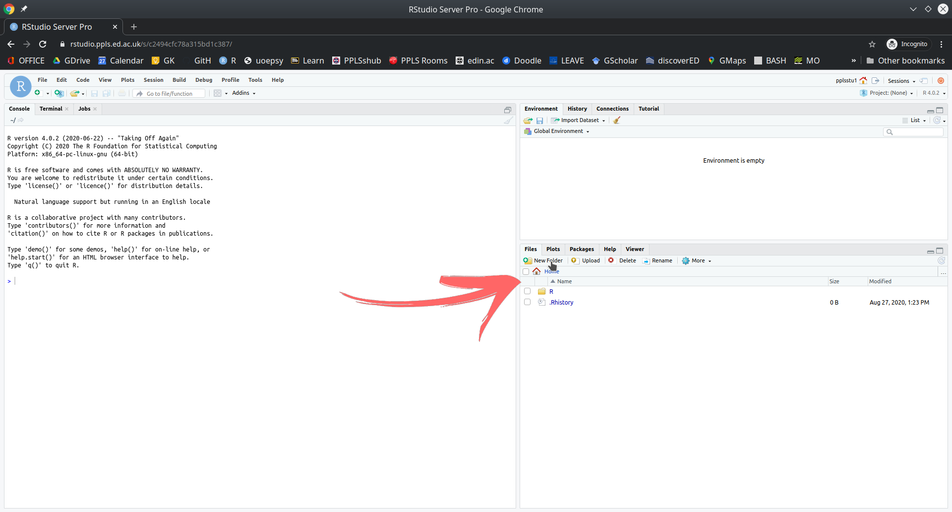
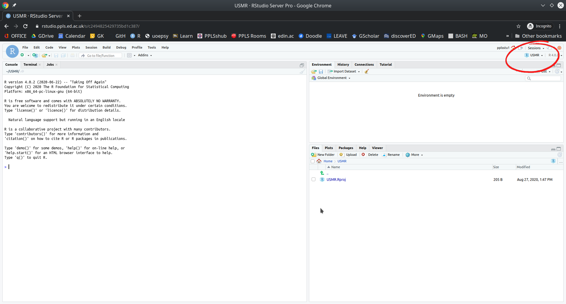
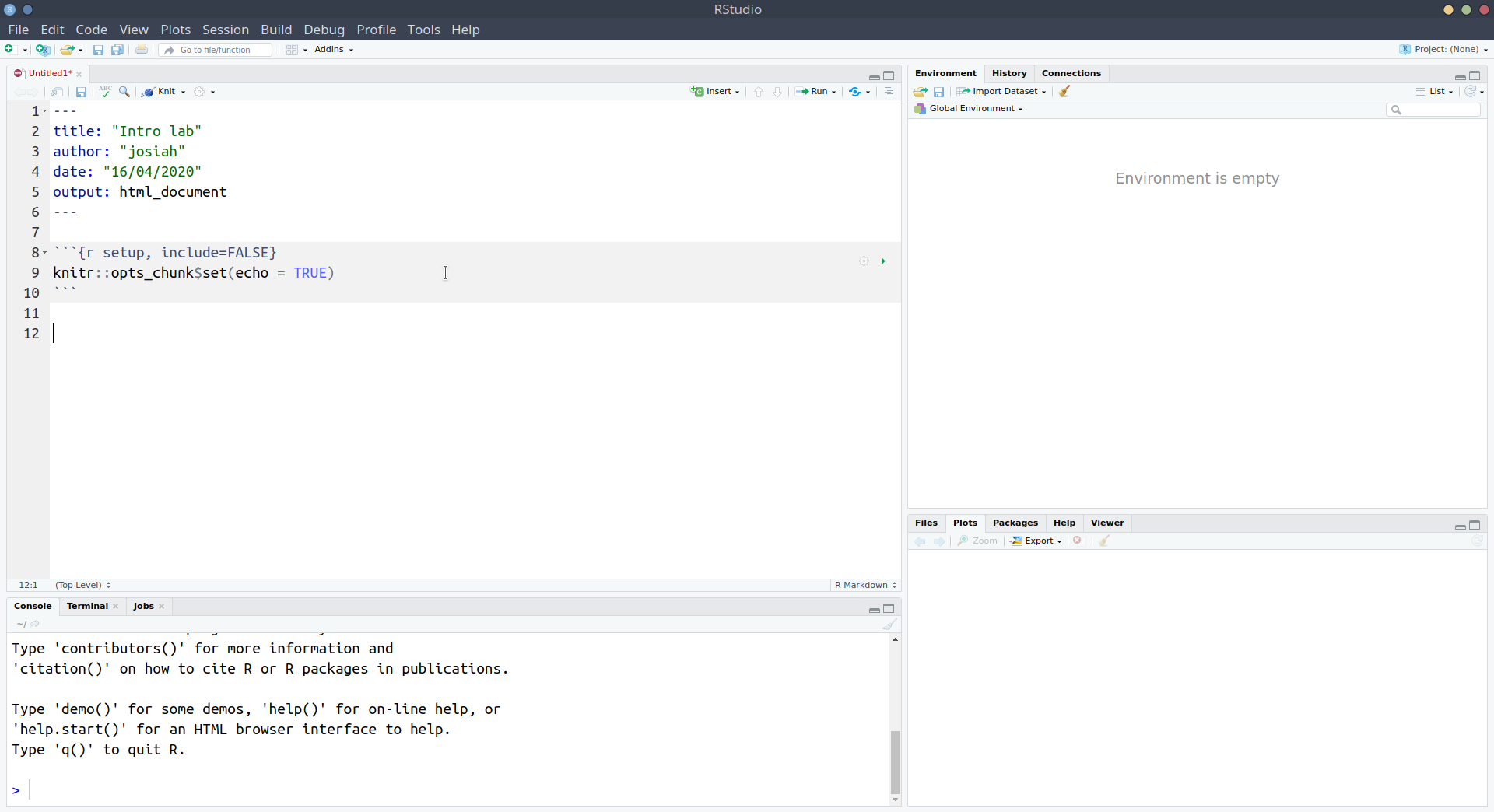
Okay, now you should have RStudio and a project open, and you should see something which looks more or less like the image below, where there are several little windows.

We are going to explore what each of these little windows offer by just diving in and starting to do things.

2.1 R as a calculator

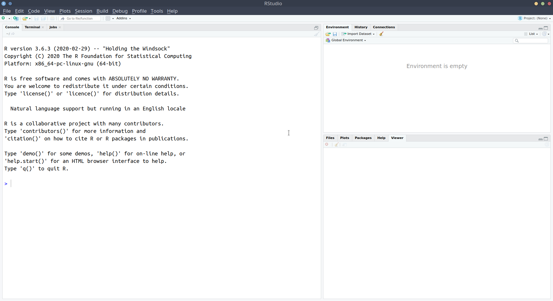
Starting in the left-hand window, you’ll notice the blue sign > which is where we R code gets executed.

Type 2+2, and hit Enter ↵. You should discover that R is a calculator.

Let’s work through some of the basic operations (adding, subtracting, etc). Try these commands yourself:

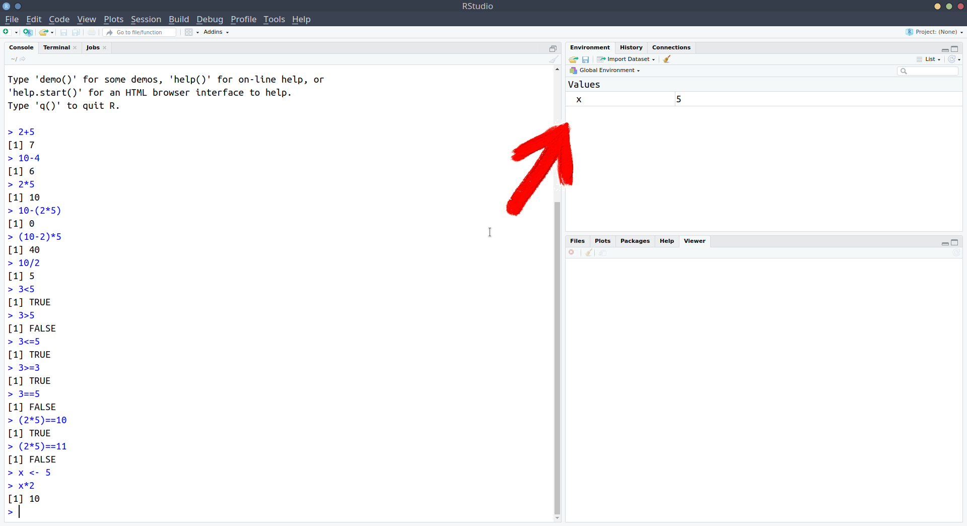
2 + 5
10 - 4
2 * 5
10 - (2 * 5)
(10 - 2) * 5
10 / 2
3^2 (Hint, interpret the ^ symbol as “to the power of”)

Whenever you see the blue sign >, it means R is ready and waiting for you to provide a command.

If you type 10 + and press Enter, you’ll see that instead of a blue > you are left with a blue +. This means that R is waiting for more. Either give it more, or cancel the command by pressing the escape key on your keyboard.

As well as performing calculations, we can ask R things, such as “Is 3 less than 5?”:

3 < 5

[1] TRUE

As the computation above returns TRUE, we notice that such questions return either TRUE or FALSE. These are not numbers and are called logical values.

Try the following:

3 > 5 “is 3 greater than 5?”
3 <= 5 “is 3 less than or equal to 5?”
3 >= 3 “is 3 greater than or equal to 3?”
3 == 5 “is 3 equal to 5?”
(2 * 5) == 10 “is 2 times 5 equal to 10?”
(2 * 5) != 11 “is 2 times 5 NOT equal to 11?”

2.2 R as a calculator with a memory

We can also store things in R’s memory, and to do that we just need to give them a name. Type x <- 5 and press Enter.

What has happened? We’ve just stored something named x which has the value 5. We can now refer to the name and it will give us the value! Try typing x and hitting Enter. It should give you the number 5. What about x * 3?

:::{.callout-info} #### Storing things in R

The <- symbol, pronounced arrow, is used to assign a value to a named object:

[name] <- [value]

Note, there are a few rules about names in R:

No spaces - spaces inside a name are not allowed (the spaces around the <- don’t matter):
- lucky_number <- 5 ✔ lucky number <- 5 ❌
Names must start with a letter:
- lucky_number <- 5 ✔ 1lucky_number <- 5 ❌
Case sensitive:
- lucky_number is different from Lucky_Number
Reserved words - there is a set of words you can’t use as names, including: if, else, for, in, TRUE, FALSE, NULL, NA, NaN, function
(Don’t worry about remembering these, R will tell you if you make the mistake of trying to name a variable after one of these).

You might have noticed that something else happened when you executed the code x <- 5. The thing we named x with a value of 5 suddenly appeared in the top-right window. This is known as the environment, and it shows everything that we store things in R:

We’ve now used a couple of the windows - we’ve been executing R code in the console, and learned about how we can store things in R’s memory (the environment) by assigning a name to them:

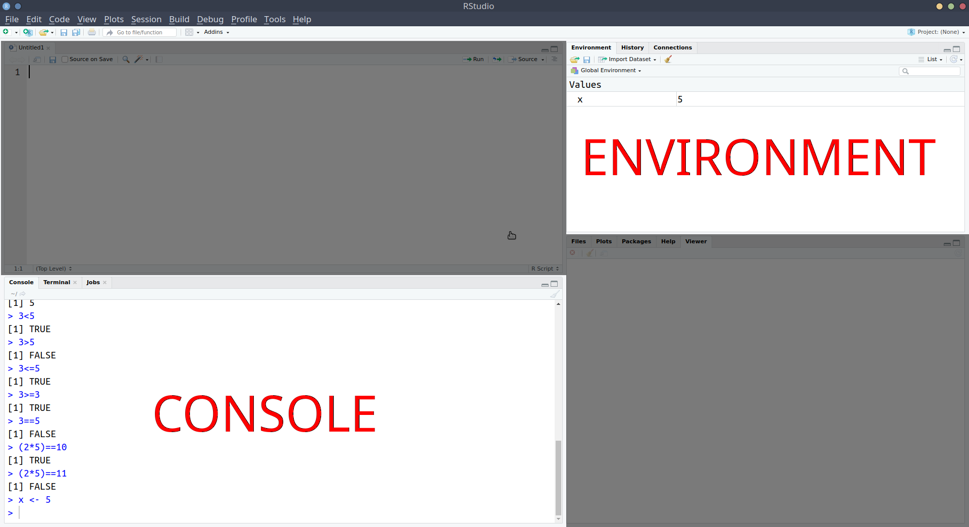
Notice that in the screenshot above, we have moved the console down to the bottom-left, and introduced a new window above it. This is the one that we’re going to talk about next.

3 R scripts and Rmarkdown

What if we want to edit our code? Whatever we write in the console just disappears upwards. What if we want to change things we did earlier on?

Well, we can write and edit our code in a separate place before sending it to the console to be executed!!

3.1 R scripts

Task

Open an R script
- File > New File > R script
Copy and paste the following into the R script

x <- 210
y <- 15
x / y

Position your text-cursor (blinking vertical line) on the top line and press:
- Ctrl + Enter on Windows
- Cmd + Enter on macOS

Notice what has happened - it has sent the command x <- 210 to the console, where it has been executed, and x is now in your environment. Additionally, it has moved the text-cursor to the next line.

Task

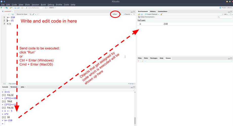
Press Ctrl + Enter (Windows) or Cmd + Enter (macOS) again. Do it twice (this will run the next two lines).

Then, change x to some other number in your R script, and run the lines again (starting at the top).

Task

Add the following line to your R script and execute it (send it to the console pressing Ctrl/Cmd + Enter):

plot(1,5)

A very basic plot should have appeared in the bottom-right of RStudio. The bottom-right window actually does some other useful things.

Task

Save the R script you have been working with:
- File > Save
- give it an appropriate name, and click save.
Check that you can now see that file in the file pane, by clicking on the “Files” tab of the bottom-right window.

NOTE: When you save R script files, they terminate with a .R extension.

3.2 Rmarkdown

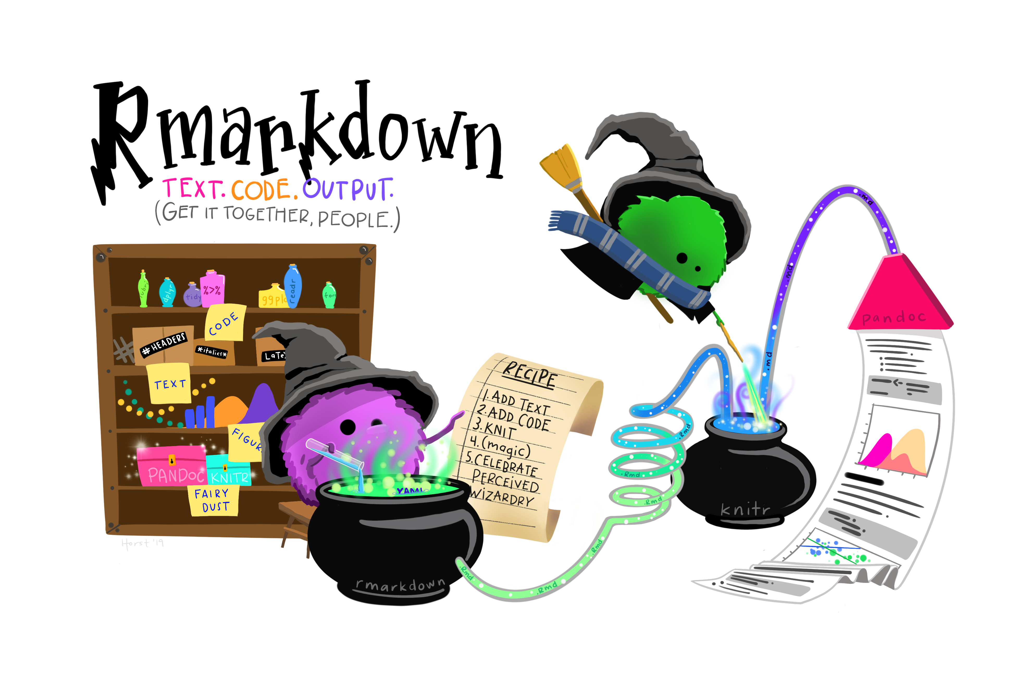
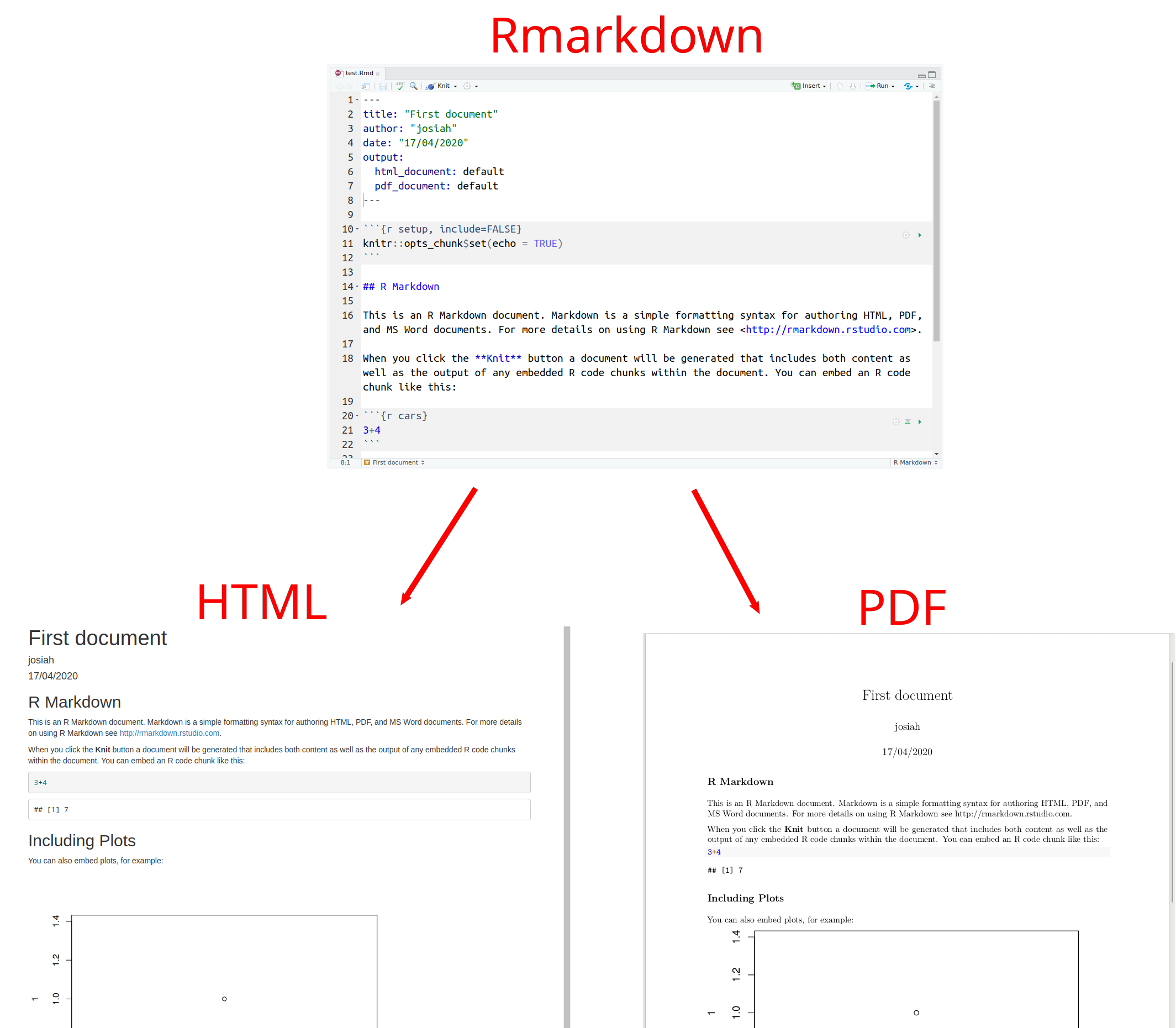
In addition to R scripts, there is another type of document we can create, known as an “Rmarkdown”.

Rmarkdown documents combine the analytical power of R and the utility of a text-processor. We can have one document which contains all of our analysis as well as our written text, and can be compiled into a nicely formatted report. This saves us doing analysis in R and copying results across to Microsoft Word. It ensures our report accurately reflects our analysis. Everything that you’re reading now has all been written in Rmarkdown!

We’re going to use Rmarkdown documents throughout this course. We’ll get into it how to write them lower down, but it basically involves writing normal text interspersed with “code-chunks” (i.e., chunks of code!). In the example below, you can see the grey boxes indicating the R code, with text in between. We can then compile the document into either a .pdf or a .html file.

4 Recap

Okay, so we’ve now seen all of the different windows in RStudio in action:

The console is where R code gets executed
The environment is R’s memory, you can assign something a name and store it here, and then refer to it by name in your code.
The editor is where you can write and edit R code and Rmarkdown documents. You can then send this to the console for it to be executed.
The bottom-right window shows you the plots that you create, the files in your project, and some other things (we’ll get to these later).

5 Take a breather

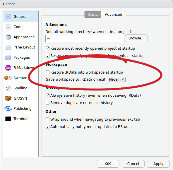
Below are a couple of our recommended settings for you to change as you begin your journey in R. After you’ve changed them, take a 5 minute break before moving on to learning about how we store data in R.

Useful Settings 1: Clean environments

As you use R more, you will store lots of things with different names. Throughout this course alone, you’ll probably name hundreds of different things. This could quickly get messy within our project.

We can make it so that we have a clean environment each time you open RStudio. This will be really handy.

In the top menu, click Tools > Global Options…
Then, untick the box for “Restore .RData into workspace at startup”, and change “Save workspace to .RData on exit” to Never:

Useful Settings 2: Wrapping code

In the editor, you might end up with a line of code which is really long, but you can make RStudio ‘wrap’ the line, so that you can see it all, without having to scroll:

x <- 1+2+3+6+3+45+8467+356+8565+34+34+657+6756+456+456+54+3+78+3+3476+8+4+67+456+567+3+34575+45+2+6+9+5+6

In the top menu, click Tools > Global Options…
In the left menu of the box, click “Code”
Tick the box for “Soft-wrap R source files”

6 R Packages

6.1 Installing R packages

Alongside the basic installation of R and RStudio, there are many add-on packages which the R community create and maintain.

The thousands of packages are part of what makes R such a powerful and useful tool - there is a package for almost everything you could want to do in R.

Task

In the console, type install.packages("cowsay") and hit Enter.

Lots of red text will come up, and it will take a bit of time.

When it has finished, and R is ready for you to use again, you will see the blue sign >.

6.2 Using R packages

It’s not enough just to install a package - to actually use the package, we need to load it using library().
We install a package only once. But each time we open RStudio, we have to load the packages we need.

Task

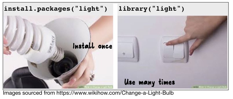
In the console again, type library(cowsay) and hit enter. This loads the package for us to use it.
Then, type say("hello world", by = "cow") and hit enter.
Hopefully you got a similar result to ours:

library(cowsay)
say("Hi Folks!", by = "cow")


 ----- 
Hi Folks! 
 ------ 
    \   ^__^ 
     \  (oo)\ ________ 
        (__)\         )\ /\ 
             ||------w|
             ||      ||

7 Your first .Rmd file

In order to be able to write and compile Rmarkdown documents (and do a whole load of other things which we are going to need throughout the course) we are now going to install a set of packages known collectively as the “tidyverse” (this includes the “rmarkdown” package).

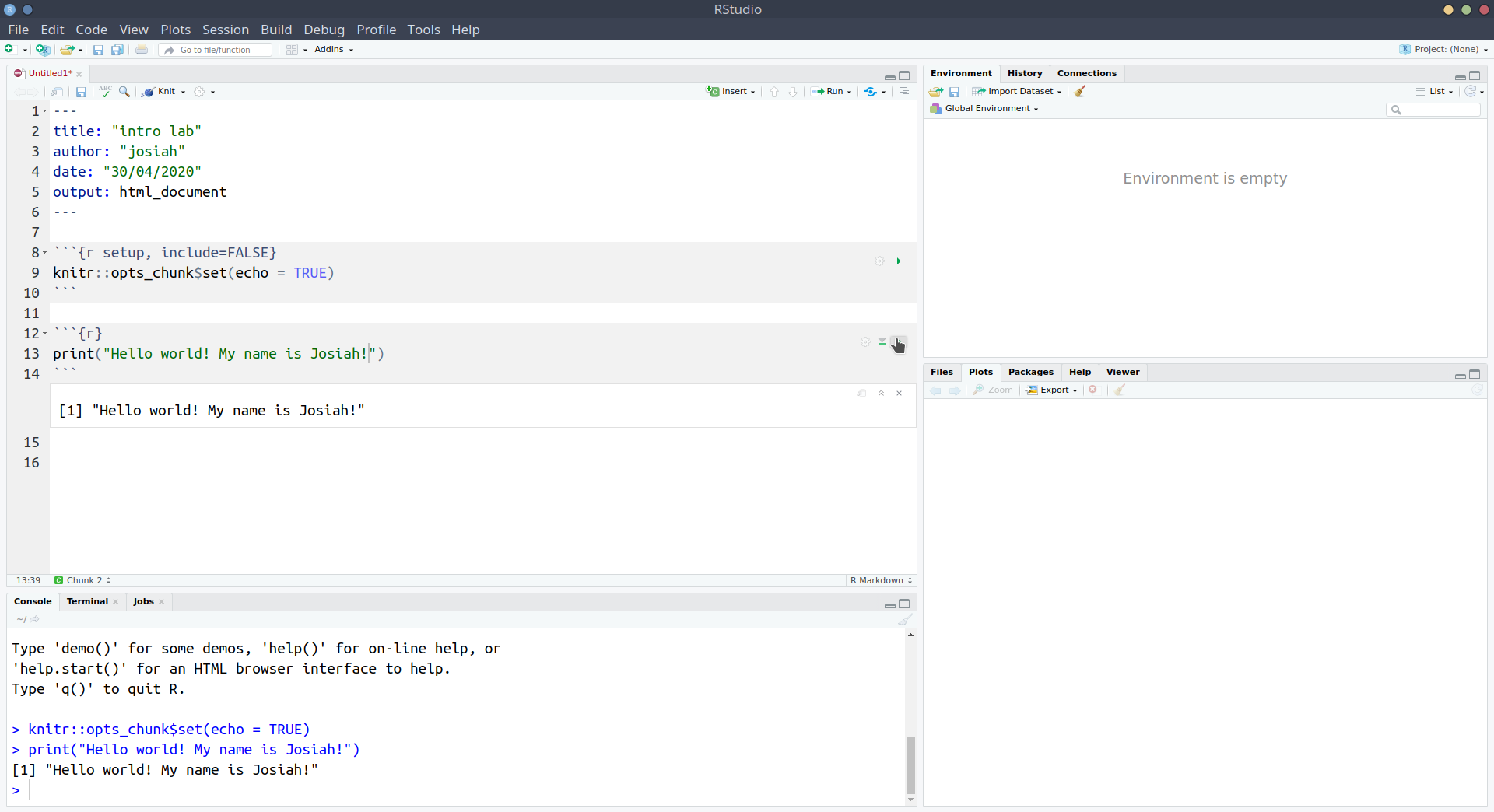
If you installed R/Rstudio on your own computer, then in the console, type install.packages("tidyverse") and hit Enter. You may have to wait a while.
If you are using rstudio.ppls.ed.ac.uk, then we have already installed “tidyverse” and a few other useful packages for you, so you don’t have to do anything!

Task

Open a new Rmarkdown document: File > New File > R Markdown…

When the box pops-up, give a title of your choice (“Intro lab”, maybe?) and your name as the author.

7.1 Writing code in a .Rmd file

The file which you have just created will have some template stuff in it. Delete everything below the first code chunk to start with a fresh document:

Task

Insert a new code chunk by either using the Insert button in the top right of the document and selecting R, or by typing Ctrl + Alt + i on Windows or Option + Cmd + i on MacOS.

Inside the chunk, type:

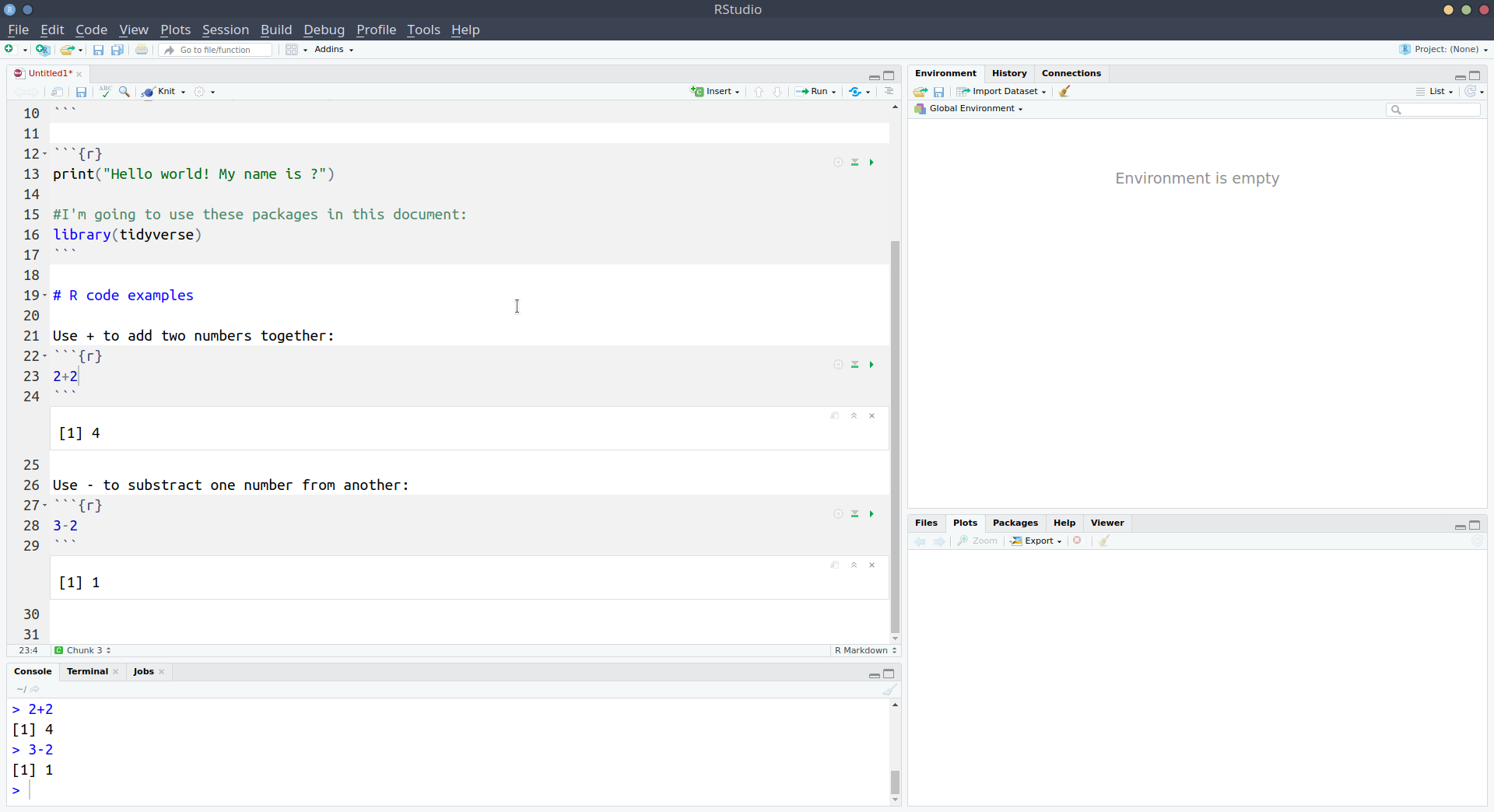
print("Hello world! My name is ?")

To execute the code inside the chunk, you can either:

do as you did in the R script - put the text-cursor on the first line, and hit Ctrl/Cmd + Enter to run the lines sequentially;
click the little green arrow at the top right of your code-chunk to run all of the code inside the chunk;
while your cursor is inside the code chunk, press Cmd + Shift + Enter to run all of the code inside the chunk.

You can see that the output gets printed below.

We’re going to use some functions which are in the tidyverse package, which we already installed above (or which we installed for you on the server).
To use the package, we need to load it.

When writing analysis code, we want it to be reproducible - we want to be able to give somebody else our code and the data, and ensure that they can get the same results. To do this, we need to show what packages we use.
It is good practice to load any packages you use at the top of your code, so that users of your code will know what packages they will need to install to run your code.

In your first code chunk, type:

# I'm going to use these packages in this document:
library(tidyverse)

and run the chunk.

NOTE: You might get various messages popping up below when you run this chunk, that is fine.

Comments in code
Note that using # in R code makes that line a comment, which basically means that R will ignore the line. Comments are useful for you to remind yourself of what your code is doing.

7.2 Writing text in a .Rmd file

Place your cursor outside the code chunk, and below the code chunk add a new line with the following:

# R code examples

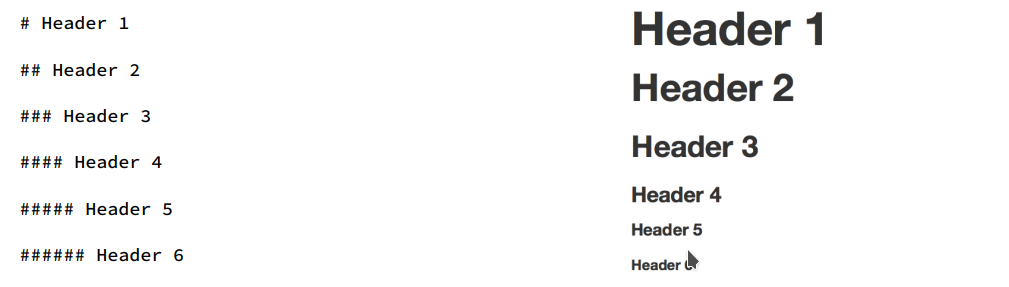
Note that when the # is used in a Rmarkdown file outside of a code-chunk, it will make that line a heading when we finally get to compiling the document. Below, what you see on the left will be compiled to look like those on the right:

7.2.1 RECALL:

Inside a code-chunk, one or more #s will create a comment
Outside a code-chunk, one ore more #s will create headings

In your Rmarkdown document, choose a few of the symbols below, and write an explanation of what it does, giving an example in a code chunk. You can see an example of the first few below.

+
-
*
/
()
^
<-
<
>
<=
>=
==
!=

7.3 Storing data into R

We’ve already seen how to assign a value to a name/symbol using <-. However, we’ve only seen how to assign a single number, e.g, x <- 5.

To store a sequence of numbers into R, we combine the values using the combine function c() and give the sequence a name. A sequence of elements all of the same type is called a vector. To view the stored content, simply type the name of the vector.

myfirstvector <- c(1, 5, 3, 7)
myfirstvector

[1] 1 5 3 7

We can perform arithmetic operations on each value of the vector. For example, to add five to each entry:

myfirstvector + 5

[1]  6 10  8 12

Recall that vectors are sequences of elements all of the same type. They do not have to be always numbers; they could be words such as real or fictional animals. Words need to be written inside quotations, e.g. “anything”, and instead of being of numeric type, we say they are characters.

wordsvector <- c("cat", "dog", "parrot", "peppapig")
wordsvector

[1] "cat"      "dog"      "parrot"   "peppapig"

NOTE

You can use either double-quote or single-quote:

c("cat", "dog", "parrot", "peppapig")

[1] "cat"      "dog"      "parrot"   "peppapig"

c('cat', 'dog', 'parrot', 'peppapig')

[1] "cat"      "dog"      "parrot"   "peppapig"

The function class() will tell you the type of the object. In this case, it is a character vector.

class(wordsvector)

[1] "character"

It does not make sense to add a number to words, hence some operations like addition and multiplication are only defined on vectors of numeric type. If you make a mistake, R will warn you with a red error message.

wordsvector + 5

Error in wordsvector + 5 : non-numeric argument to binary operator

Finally, it is important to notice that if you combine together in a vector a number and a word, R will transform all elements to be of the same type. Why? Recall: vectors are sequences of elements all of the same type. Typically, R chooses the most general type between the two. In this particular case, it would make everything a character, check the ““, as it would be harder to transform a word into a number!

mysecondvector <- c(4, "cat")
mysecondvector

[1] "4"   "cat"

7.4 Reading data into R

While we can manually input data like we did above, more often, we will need to read in data which has been created elsewhere (like in excel, or by some software which is used to present participants with experiments).

Task

Add a new heading by typing the following:

# Reading and storing data

Remember: We make headings using the # outside of a code chunk.

Task

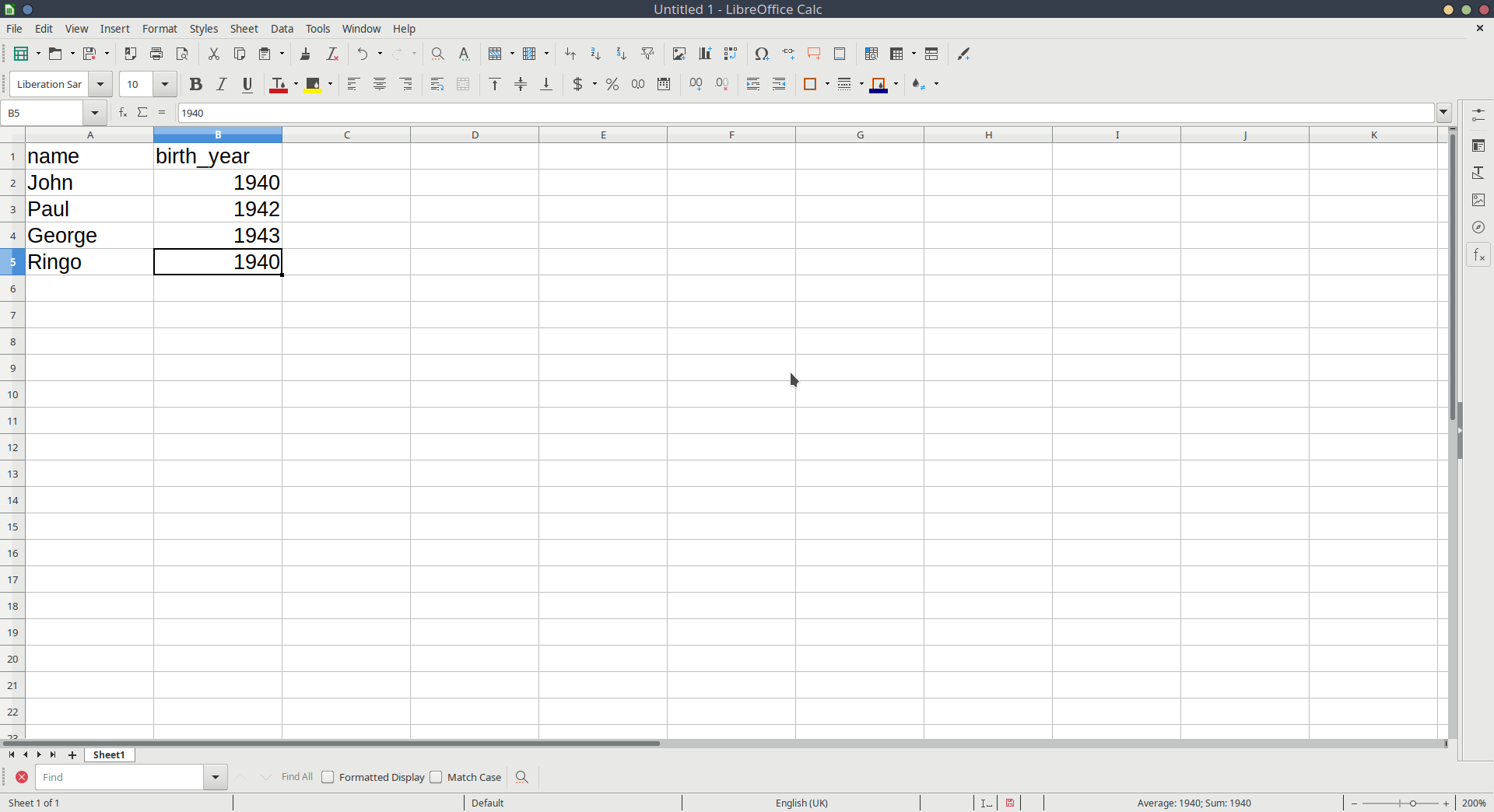
Open Microsoft Excel, or LibreOffice Calc, or whatever spreadsheet software you have available to you, and create some data with more than one variable.

It can be whatever you want, but we’ve used a very small example here for you to follow, so feel free to use it if you like.

We’ve got two sets of values here: the names and the birth-years of each member of the Beatles. The easiest way to think of this would be to have a row for each Beatle, and a column for each of name and birth-year.

Task

Save the data as a .csv file.

Although R can read data when it’s saved in Microsoft/LibreOffice formats, the simplest, and most universal way to save data is as simple text, with the values separated by some character - .csv stands for comma separated values.

In Microsoft Excel, if you go to File > Save as

In the Save as Type box, choose to save the file as CSV (Comma delimited).

Important: save your data in the project folder you created at the start of this lab.

Back in RStudio…

Next, we’re going to read the data into R. We can do this by using the read_csv() function, and directing it to the file you just saved.

If you are using RStudio on the server, you will need to upload the file you just saved to the server. The video below shows an example of this:

Task

Create a new code-chunk in your Rmarkdown and, in the chunk, type: read_csv("name-of-your-data.csv"), where you replace name-of-your-data with whatever you just saved your data as in your spreadsheet software.

Helpful tip
If you have your text-cursor inside the quotation marks, and press the tab key on your keyboard, it will show you the files inside your project. You can then use the arrow keys to choose between them and press Enter to add the code:

When you run the line of code you just wrote, it will print out the data, but will not store it. To do that, we need to assign it as something:

beatles <- read_csv("data_from_excel.csv")

Note that this will now turn up in the Environment pane of RStudio.

Now that we’ve got our data in R, we can print it out by simply invoking its name:

beatles

# A tibble: 4 × 2
  name   birth_year
  <chr>       <dbl>
1 John         1940
2 Paul         1942
3 George       1943
4 Ringo        1940

And we can do things such as ask R how many rows and columns there are:

dim(beatles)

[1] 4 2

This says that there are 4 members of the Beatles, and for each we have 2 measurements.

To get more insight into what the data actually are, you can either use the structure str() function, or glimpse() function to get a glimpse at the data:

str(beatles)

spc_tbl_ [4 × 2] (S3: spec_tbl_df/tbl_df/tbl/data.frame)
 $ name      : chr [1:4] "John" "Paul" "George" "Ringo"
 $ birth_year: num [1:4] 1940 1942 1943 1940
 - attr(*, "spec")=
  .. cols(
  ..   name = col_character(),
  ..   birth_year = col_double()
  .. )
 - attr(*, "problems")=<externalptr>

glimpse(beatles)

Rows: 4
Columns: 2
$ name       <chr> "John", "Paul", "George", "Ringo"
$ birth_year <dbl> 1940, 1942, 1943, 1940

Task

Use dim() to confirm how many rows and columns are in your data.

Use str() or glimpse() to take a look at the structure of the data. Don’t worry about the output of str() right now, we’ll pick up with this in the next chapter.

7.5 Getting help in R

dim(), str(), read_csv() are all functions.

Functions perform specific operations / transformations in computer programming.

They can have inputs and outputs. For example, dim() takes some data you have stored in R as its input, and gives the dimensions of the data as its output.

In R, functions come with help pages, where you can see information about the various inputs and outputs, and examples of how to use them.

In the console, type ?dim (or ?dim() will work too) and press Enter.
The bottom-right pane (where things like plots are also shown), should switch to the Help tab, and open the documentation page for the dim() function!

Why did we ask you to write this bit in the console, whereas previously we’ve been writing stuff in the RMarkdown document in the editor?

Well, when writing an RMarkdown document, the aim at the end is to have a nice document which we can read. For instance, we can write statistical reports, journal papers, coursework reports etc, in Rmarkdown. But the reader doesn’t need to see that we’re looking up how to use some function - just like they don’t need to know that we might look up a word in the dictionary before using it.

7.6 Compiling a .Rmd file

Task

By now, you should have an Rmardkown document (.Rmd) with your answers to the tasks we’ve been through today.

Compile the document by clicking on the Knit button at the top (it will ask you to save your document first). The little arrow to the right of the Knit button allows you to compile to either .pdf or .html.

8 Checklist for today

EITHER:
- Option A: Get started with the PPLS RStudio Server ✔
- Option B: Install R and RStudio ✔
Start a new project for the course ✔
Change a few RStudio settings (recommended) ✔
Install some R packages (the “tidyverse”) ✔
Create a new Rmarkdown document ✔
Complete today’s tasks and exercises on storing data in R ✔
Compile your Rmarkdown document ✔
Celebrate! ✔ 🎉

9 Glossary

Console: where the code gets executed
Environment: R’s memory, it lists all the names of things with stuff stored into them
Editor: where we edit code
R script: a file with R code and comments
Rmarkdown document: an enhanced file where you can combine together R code, explanatory text, and plots.
packages (also library): user-created bundles providing additional functionality to your local R installation
functions: they take inputs, do some transformation or computation on them, and return a result (output)
?: returns the help page of a function, e.g. ?dim.

Symbol	Description	Example
`+`	Adds two numbers together	`2+2` - two plus two
`-`	Subtract one number from another	`3-1` - three minus one
`*`	Multiply two numbers together	`3*3` - three times three
`/`	Divide one number by another	`9/3` - nine divided by three
`()`	group operations together	`(2+2)/4` is different from `2+2/4`
`^`	to the power of..	`4^2` - four to the power of two, or four squared
`<-`	stores an object in R with the left hand side (LHS) as the name, and the RHS as the value	`x <- 10`
`=`	stores an object in R with the left hand side (LHS) as the name, and the RHS as the value	`x = 10`
`<`	is less than?	`2 < 3`
`>`	is greater than?	`2 > 3`
`<=`	is less than or equal to?	`2 <= 3`
`>=`	is greater than or equal to?	`2 >= 2`
`==`	is equal to?	`(5+5) == 10`
`!=`	is not equal to?	`(2+3) != 4`
`c()`	combines values into a vector (a sequence of values)	`c(1,2,3,4)`