| Variable | Description |
|---|---|
| type | College Type: −1 = Not reported; 1 = Public; 2 = Private for-profit; 3 = Private not-for-profit (no religious affiliation); 4 = Private not-for-profit (religious affiliation) |
| region | Region: 0 = US Service schools; 1 = New England; 2 = Mid East; 3 = Great Lakes; 4 = Plains; 5 = Southeast; 6 = Southwest; 7 = Rocky Mountains; 8 = Far West; 9 = Outlying areas |
| gradrate | Graduation Rate – All |
| gradratem | Graduation Rate – Men |
| gradratew | Graduation Rate – Women |
Hypothesis testing and confidence intervals
Semester 2 - Week 4
Next week: submission of Formative Report C (PDF file only)
You are required to submit a PDF file by 12 noon on Friday the 17th of February 2023 via Learn. One person needs to submit on behalf of your group.
No extensions allowed. As this is group-based work, no extensions are possible.
-
The report should be at most 6 pages long. At the end of the report, you are allowed two appendices which don’t count towards the page limit.
- Appendix A will contain any tables or figures which you cannot fit in the page limit (no text allowed).
- Appendix B will contain the code to reproduce the report results.
Excluding Appendix B, the report should only include text, figures or tables. It should not include any reference to R code or functions, but be written for a generic reader who is only assumed to have a basic statistical understanding without any R knowledge. You should also avoid any R code output or printout in the PDF file.
The report title should be “Formative Report C (Group 0.A)”. Replace Group 0.A to be your group name.
-
In the author section of the PDF file write the exam number of each person within the group. The exam number starts with the letter B and can be found on your student ID card.
- For example: B000001, B000002, B000003, B000004
You will receive formative feedback on your submission during Flexible Learning Week. Please keep going to the labs that week in order to receive feedback.
Are you registered for your group on Learn?
Go to the course Learn page, on the left-hand side click “Groups information”, then the lab, and then the group name. Click Sign up.
1 Tasks
The data dataset-ipeds-2012-subset2, available at https://uoepsy.github.io/data/dataset-ipeds-2012-subset2.csv, is a subset of data derived from the Integrated Postsecondary Education Data System (IPEDS) at the National Center for Education Statistics, 2012. The data were collected for a random sample from all colleges and universities in the United States in that year. The variables include:
In formative report C, you will investigate the mean graduation rate for female students at colleges and universities in the United States. Specifically, you are asked to perform the following tasks, each related to a week of teaching in this course.
This week you will only focus on task C4.
C1) Read the data into R, describe the variable of interest both visually and numerically, and provide a 95% CI for the mean graduation rate of female students at colleges and universities in the United States.
C2) At the 5% significance level and using the p-value method, test whether the mean graduation rate for female students at colleges and universities in the United States is significantly different from a rate of 50 percent.
C3) At the 5% significance level and using the critical value method, test whether the mean graduation rate for female students at colleges and universities in the United States is significantly different from a rate of 50 percent.
This week’s task
C4) Tidy up your report so far, making sure to have 3 sections: introduction, analysis and discussion. After those, you can have Appendix A (additional figures or tables) and Appendix B (the R code used).
C5) Compute and report the effect size, check if the assumptions underlying the t-test are violated.
2 C4 sub-tasks
In this section you will find some guided sub-steps you may want to consider to complete task C4.
Tip
To see the hints, hover your cursor on the superscript numbers.
- Reopen last week’s Rmd file, as you will continue last week’s work and build on it.1
-
Ensure that your report has 3 sections:
- Introduction - where you provide a brief description of the data, variables and their type, and the research questions you are going to address.
- Analysis - where you show and describe your results. Please note that no R code or output should be visible, but only figures and tables.
- Discussion - where you summarise your key results in a few take-home messages that answer the research questions.
Structure your Rmd file as follows:
---
title: "Formative report C (Group 0.A)"
author: "B000000, B000001, B00002, B00003, B000004"
date: "Write the date here"
output: bookdown::pdf_document2
toc: false
---
This is the metadata block. It includes the:
- document title
- author name
- date (to leave empty, use an empty string
"") - the output type
The output type could be html_document, pdf_document, etc.
We use bookdown::pdf_document2 so that we can reference figures, which pdf_document doesn’t let you do.
The code bookdown::pdf_document2 simply means to use the pdf_document2 type from the bookdown package.
The code toc: false hides the table of contents.
```{r setup, include=FALSE}
knitr::opts_chunk$set(echo=FALSE, message=FALSE, warning=FALSE)
```
This is the setup chunk and should always be included in your Rmd document. It sets the global options for all code chunks that will follow.
- If
echo=TRUE, the R code in chunks is displayed. If FALSE, not. - If
message=TRUE, information messages are displayed. If FALSE, not. - If
warning=TRUE, warning messages are printed. If FALSE, not.
If you want to change the setting in a specific code chunk, you can do so via:
```{r, echo=FALSE}
# A code chunk
```
```{r, include=FALSE}
# week 1 code below
library(tidyverse)
# week 2 code below
pltEye <- ggplot(starwars, aes(x = eye_color)) +
geom_bar()
# week 3 code below
# week 4 code below
# week 5 code below
```This code chunks contains your rough work from each week. Give names to plots and tables, so that you can reference those later on. The option include=FALSE hides both code and output.
To run each line of code while you are working, put your cursor on the line and press Control + Enter on Windows or Command + Enter on a macOS.
## Introduction

Write here an introduction to the data, the variables, and anything worth of
notice in the data.


## Analysis

Present here your tables, plots, and results. In the code chunk below, you do
not need to put the chunk option `echo=FALSE` as you set this option globally
in the setup chunk.

```{r}
pltEye
```

If you didn't set it globally, you would need to put it in the chunk options:

```{r, echo=FALSE}
pltEye
```

More text...


## Discussion

Write up your take home messages here...
This contains your actual textual reporting, as well as tables and figures. To show in place a plot previously created, just include the plot name in a code chunk with the option echo = FALSE to hide the code but display the output.
## Appendix A - Additional tables and figures

Insert here any additional tables or figures that you could not fit in the
page limit.
## Appendix B - R code
```{r ref.label=knitr::all_labels(), echo=TRUE, eval=FALSE}
```Copy and paste in your report this last code chunk as it is here. This special code chunk will copy here all the previous R code chunks that you have created and automatically populate Appendix B for you.
Note
The appendices do not count towards the 6-page limit.
3 Worked Example
The R code is visible here for instructional purposes only, but it should not be visible in a PDF report. It should only appear as part of the appendix.
R code
library(tidyverse)
library(patchwork)
library(kableExtra)

pass_scores <- read_csv("https://uoepsy.github.io/data/pass_scores.csv")
dim(pass_scores)
head(pass_scores)
glimpse(pass_scores)

summary(pass_scores)

plt_hist <- ggplot(pass_scores, aes(x = PASS)) +
    geom_histogram(color = 'white') +
    labs(x = "PASS scores", title = "(a) Histogram")

plt_box <- ggplot(pass_scores, aes(x = PASS)) +
    geom_boxplot() +
    labs(x = "PASS scores", title = "(b) Boxplot")

plt_hist / plt_box
stats <- pass_scores %>%
summarise(n = n(),
Min = min(PASS),
Max = max(PASS),
M = mean(PASS),
SD = sd(PASS))
kbl(stats, booktabs = TRUE, digits = 2,
caption = "Descriptive statistics for PASS scores")
# Confidence interval
xbar <- stats$M
s <- stats$SD
n <- stats$n
se <- s / sqrt(n)
tstar <- qt(c(0.025, 0.975), df = n - 1)
xbar + tstar * se
# observed t-statistic
tobs <- (xbar - 33) / se
tobs
# p-value method
pvalue <- 2 * pt(abs(tobs), df = n - 1, lower.tail = FALSE)
pvalue
# critical value method
tstar
tobs
Introduction
A random sample of 20 students from the University of Edinburgh completed a questionnaire measuring their total endorsement of procrastination. The data, available from https://uoepsy.github.io/data/pass_scores.csv, were used to estimate the average procrastination score of all Edinburgh University students, as well as testing whether the mean procrastination score differed from the Solomon & Rothblum reported average of 33 at the 5% significance level. The recorded variables include a subject identifier (sid, categorical), the school each belongs to (school, categorical), and the total score on the Procrastination Assessment Scale for Students (PASS, numeric). The data do not include any impossible values for the PASS scores, as they were all within the possible range of 0 – 90. To answer the questions of interest, in the following we will only focus on the total PASS score variable.
Analysis
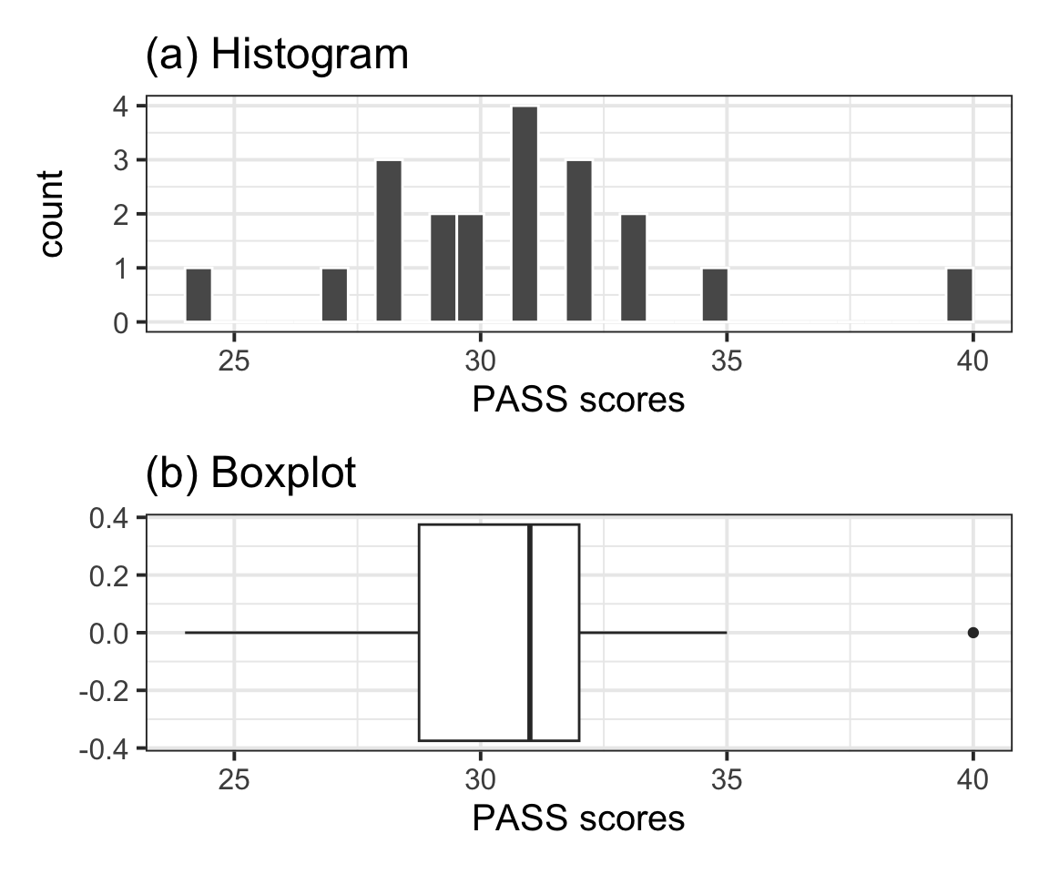
The distribution of PASS scores, as shown in Figure 1(a), is roughly bell shaped and does not have any impossible values. The outlier (40) depicted in the boxplot shown in Figure 1(b) is well within the range of plausible values for the PASS scale (0–90) and as such was not removed for the analysis.
| n | Min | Max | M | SD |
|---|---|---|---|---|
| 20 | 24 | 40 | 30.7 | 3.31 |
Table 1 displays summary statistics for the PASS scores in the sample of Edinburgh University students. From the sample data we obtain an average procrastination score of \(M = 30.7\), 95% CI [29.15, 32.25]. Hence, we are 95% confident that a Edinburgh University student will have a procrastination score between 29.15 and 32.25, which is between 0.75 and 3.85 lower than the average score of 33 reported by Solomon & Rothblum.
Let \(\mu\) denote the mean PASS score of all Edinburgh University students. At the 5% significance level, we performed a one sample t-test of \(H_0 : \mu = 33\) against \(H_1 : \mu \neq 33\). The sample data provide very strong evidence against the null hypothesis and in favour of the alternative one that the mean procrastination score of Edinburgh University students is significantly different from the Solomon & Rothblum reported average of 33: \(t(19) = -3.11, p = .006\), two-sided.
Discussion
Data including the Procrastination Assessment Scale for Students (PASS) scores for a random sample of 20 students at Edinburgh University we used to estimate the average procrastination score for a student of that university. In addition, the data were used to test whether there is a significant difference between that average score and the Solomon & Rothblum reported average of 33.
We are 95% confident that a Edinburgh University student will have a procrastination score between 29.15 and 32.25. Furthermore, at the 5% significance level, the data provide very strong evidence that the mean procrastination score of Edinburgh University students is different from 33. The confidence interval, reported above, indicates that a Edinburgh University student tends to have a mean procrastination score between 0.75 and 3.85 lower than the Solomon & Rothblum reported average of 33.
What is missing from this instructional example:
- Appendix A
- Appendix B
Footnotes
Hint: Ask last week’s driver for the Rmd file, they should share it with the group via email or Teams. To download the file from the server, go to the RStudio Files pane, tick the box next to the Rmd file, and select More > Export.↩︎