| Variable | Description |
|---|---|
| type | College Type: −1 = Not reported; 1 = Public; 2 = Private for-profit; 3 = Private not-for-profit (no religious affiliation); 4 = Private not-for-profit (religious affiliation) |
| region | Region: 0 = US Service schools; 1 = New England; 2 = Mid East; 3 = Great Lakes; 4 = Plains; 5 = Southeast; 6 = Southwest; 7 = Rocky Mountains; 8 = Far West; 9 = Outlying areas |
| gradrate | Graduation Rate – All |
| gradratem | Graduation Rate – Men |
| gradratew | Graduation Rate – Women |
Confidence intervals
Semester 2 - Week 1
1 Formative Report C instructions
Formative report C - Instructions
In the next five weeks of the course you should produce a PDF report using Rmarkdown for which you will receive formative feedback in Flexible Learning Week.
The report should not include any reference to R code or functions, but be written for a generic reader who is only assumed to have a basic statistical understanding without any R knowledge. You should also avoid any R code output or printout in the PDF file.
You will be required to submit a PDF file by 12 noon on Friday the 17th of February 2023 via Learn. One person needs to submit on behalf of your group.
-
The report should be at most 6 pages long. At the end of the report, you are allowed two appendices which both don’t count towards the page limit.
- Appendix A will contain any tables or figures which you cannot fit in the page limit (no text allowed).
- Appendix B will contain the code to reproduce the report results.
No extensions allowed. As this is group-based work, no extensions are possible.
Are you registered for your group on Learn?
Go to the course Learn page, on the left-hand side click “Groups information”, then the lab, and then the group name. Click Sign up.
Change driver this week
In the next five weeks your group will be creating a new formative report, Formative Report C.
- Choose a driver for this week
- The driver should login to the PC provided with the desk, and access RStudio Server
- The driver is the only person allowed to type the report during this lab
- The others in the group are the navigators
- Navigators are responsible for suggesting and commenting on the strategy that the driver needs to follow to answer the tasks, as well as correct typos and coding errors.
- It is important that your group chooses a driver for this week, and in the next weeks the driver rotates every week to ensure that everyone in the group has contributed to the writing of the report.
Create a new RMD file
Create a new Rmd file for formative report C which you will build upon each week in your group.
At the end of each lab, save the Rmd file and share it with your group. If you go to your group area on Learn, you can click “Send Email” to share the file with your group.
2 Tasks
The data dataset-ipeds-2012-subset2, available at https://uoepsy.github.io/data/dataset-ipeds-2012-subset2.csv, is a subset of data derived from the Integrated Postsecondary Education Data System (IPEDS) at the National Center for Education Statistics, 2012. The data were collected for a random sample from all colleges and universities in the United States in that year. The variables include:
In formative report C, you will investigate the mean graduation rate for female students at colleges and universities in the United States. Specifically, you are asked to perform the following tasks, each related to a week of teaching in this course.
This week you will only focus on task C1.
This week’s task
C1) Read the data into R, describe the variable of interest both visually and numerically, and provide a 95% CI for the mean graduation rate of female students at colleges and universities in the United States.
C2) At the 5% significance level and using the p-value method, test whether the mean graduation rate for female students at colleges and universities in the United States is significantly different from a rate of 50 percent.
C3) At the 5% significance level and using the critical value method, test whether the mean graduation rate for female students at colleges and universities in the United States is significantly different from a rate of 50 percent.
C4) Tidy up your report so far, making sure to have 3 sections: introduction, analysis and discussion.
C5) Compute and report the effect size, check if the assumptions underlying the t-test are violated.
3 C1 sub-tasks
In this section you will find some guided sub-steps you may want to consider to complete task C1.
Tip
To see the hints, hover your cursor on the superscript numbers.
Read the data into R and inspect it.1
How many units are there?2
Visualise the distribution of the variable of interest (
gradratew). What is the shape of the distribution? Are there any outliers?3Compute and interpret a table of descriptive statistics for the variable of interest. At a minimum, ensure that it includes both a measure of centre and spread.4
Compute a 95% confidence interval for the mean graduation rate of female college students in 2012.5
For the report introduction, write a brief introduction to the data and question being investigated. How many cases are there? Is there any impossible values? What is the type of the variables and which one is used for the investigation?
Provide a write up of your results so far, using proper rounding and making sure to report your results in context of the investigation.
4 Worked Example
The Procrastination Assessment Scale for Students (PASS) was designed to assess how individuals approach decision situations, specifically the tendency of individuals to postpone decisions (Solomon & Rothblum, 1984).
The PASS assesses the prevalence of procrastination in six areas: writing a paper; studying for an exam; keeping up with reading; administrative tasks; attending meetings; and performing general tasks. For a measure of total endorsement of procrastination, responses to 18 questions (each measured on a 1-5 scale) are summed together, providing a single score for each participant (range 0 to 90). The mean score from Solomon & Rothblum, 1984 was 33.
Investigation:
What is the average procrastination score of Edinburgh University students?
To answer this question, we will use data collected for a random sample of students from the University of Edinburgh: https://uoepsy.github.io/data/pass_scores.csv
| Variable Name | Description |
|---|---|
| sid | Subject identifier |
| school | School each subject belonged to |
| PASS | Total endorsement of procrastination score |
Necessary packages:
- tidyverse for using
read_csv(), usingsummarise()andggplot(). - patchwork for arranging plots side by side or underneath
- kableExtra for creating user-friendly tables
Read the data into R:
To inspect the data:
head(pass_scores)# A tibble: 6 × 3
sid school PASS
<chr> <chr> <dbl>
1 s_1 GeoSciences 31
2 s_2 ECA 24
3 s_3 LAW 32
4 s_4 ECA 40
5 s_5 LAW 28
6 s_6 SSPS 31glimpse(pass_scores)Rows: 20
Columns: 3
$ sid <chr> "s_1", "s_2", "s_3", "s_4", "s_5", "s_6", "s_7", "s_8", "s_9", …
$ school <chr> "GeoSciences", "ECA", "LAW", "ECA", "LAW", "SSPS", "PPLS", "SLL…
$ PASS <dbl> 31, 24, 32, 40, 28, 31, 30, 28, 32, 29, 28, 33, 35, 33, 30, 31,…summary(pass_scores) sid school PASS
Length:20 Length:20 Min. :24.00
Class :character Class :character 1st Qu.:28.75
Mode :character Mode :character Median :31.00
Mean :30.70
3rd Qu.:32.00
Max. :40.00 Visualise the distribution of PASS scores:
Note
The boxplot highlights an outlier (40). However, this value is well within the plausible range of the scale (0 – 90), hence it is of no concern and the point can be kept for the analysis.
plt_hist <- ggplot(pass_scores, aes(x = PASS)) +
    geom_histogram(color = 'white')

plt_box <- ggplot(pass_scores, aes(x = PASS)) +
    geom_boxplot()

plt_hist / plt_box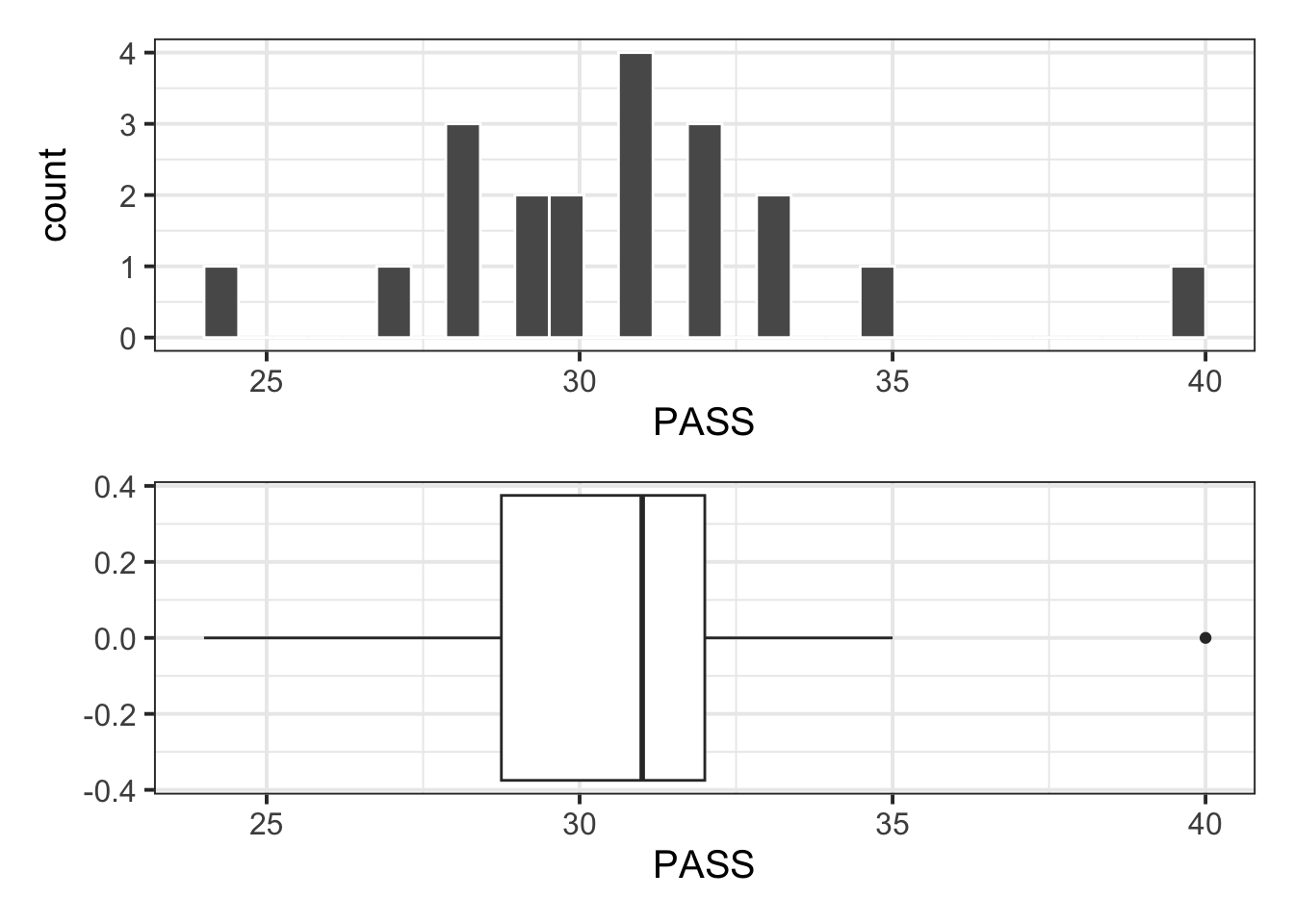
Descriptive statistics:
| n | Min | Max | M | SD |
|---|---|---|---|---|
| 20 | 24 | 40 | 30.7 | 3.31 |
When estimating a parameter, in this case the mean score on the Procrastination Assessment Scale for Students (PASS) for all Edinburgh University students, we do not just report the estimate (sample average score), but also something that reflects our uncertainty in the estimate. This can either be the standard error or a confidence interval. If asked to compute a 95% confidence interval for the mean score on the Procrastination Assessment Scale for Students (PASS) for all Edinburgh University students, we could do:
# Sample mean
xbar <- stats$M

# Standard error
s <- stats$SD
n <- stats$n
se <- s / sqrt(n)
se
[1] 0.7401991[1] -2.093024 2.093024# CI
xbar + tstar * se[1] 29.15075 32.24925WARNING!
This code won’t work if stats stores a kable, i.e. the result of kbl(). Make sure this only stores the tibble, rather than the pretty version from kbl()!
Report
These three code chunks should not be visible in the report. You can simply report the CI in a paragraph using the style [LowerCI, UpperCI].
Example introduction
A random sample of 20 students from the University of Edinburgh completed a questionnaire measuring their total endorsement of procrastination. The data, available from https://uoepsy.github.io/data/pass_scores.csv, were used to estimate the average procrastination score of all Edinburgh University students. The recorded variables included a subject identifier (sid), the school of each subject (school), and the total score on the Procrastination Assessment Scale for Students (PASS). The data do not include any impossible values for the PASS scores, as they were all within the possible range of 0 – 90. To answer the question of interest, in the following we will only focus on the total PASS score variable.
Example CI interpretation
From the sample data we obtain an average procrastination score of \(M = 30.7\), 95% CI [29.15, 32.25]. Hence, we are 95% confident that a Edinburgh University student will have a procrastination score between 29.15 and 32.25, which is between 0.75 and 3.85 lower than the average score of 33 reported by Solomon & Rothblum.
5 Student Glossary
To conclude the lab, add the new functions to the glossary of R functions.
| Function | Use and package |
|---|---|
geom_histogram |
? |
geom_boxplot |
? |
summarise |
? |
n() |
? |
mean |
? |
sd |
? |
qt |
? |
Footnotes
Hint: Some of the following functions may be useful:
read_csv()from tidyverse,head(),glimpse(),summary()↩︎Hint: Some of the following functions may be useful:
nrow(DATA),dim(DATA),length(DATA$Y),summarise(n = n())↩︎Hint:
geom_histogram(),geom_density(),geom_boxplot()may be useful functions.↩︎Hint:
summarise()from the tidyverse package ordescribe()from the psych package↩︎-
Hints:
Step 1: Compute the average gradution rate of female college students
Step 2: Compute the standard error of the mean
Step 3: Compute the quantiles of a t distribution with \(n-1\) degrees of freedom, where \(n\) = sample size, cutting a probability of 0.95 in between them.
Step 4: Obtain the confidence interval using the formula:
\[95\% \text{ CI: } \left[ \bar x - t^* SE_{\bar{x}}, \ \bar x + t^* SE_{\bar{x}} \right]\] \[\text{where} \qquad SE_{\bar{x}} = \frac{s}{\sqrt n}\]↩︎