| Variable | Description |
|---|---|
| type | College Type: −1 = Not reported; 1 = Public; 2 = Private for-profit; 3 = Private not-for-profit (no religious affiliation); 4 = Private not-for-profit (religious affiliation) |
| region | Region: 0 = US Service schools; 1 = New England; 2 = Mid East; 3 = Great Lakes; 4 = Plains; 5 = Southeast; 6 = Southwest; 7 = Rocky Mountains; 8 = Far West; 9 = Outlying areas |
| gradrate | Graduation Rate – All |
| gradratem | Graduation Rate – Men |
| gradratew | Graduation Rate – Women |
Hypothesis testing: critical values
Semester 2 - Week 3
1 Tasks
The data dataset-ipeds-2012-subset2, available at https://uoepsy.github.io/data/dataset-ipeds-2012-subset2.csv, is a subset of data derived from the Integrated Postsecondary Education Data System (IPEDS) at the National Center for Education Statistics, 2012. The data were collected for a random sample from all colleges and universities in the United States in that year. The variables include:
In formative report C, you will investigate the mean graduation rate for female students at colleges and universities in the United States. Specifically, you are asked to perform the following tasks, each related to a week of teaching in this course.
This week you will only focus on task C3.
C1) Read the data into R, describe the variable of interest both visually and numerically, and provide a 95% CI for the mean graduation rate of female students at colleges and universities in the United States.
C2) At the 5% significance level and using the p-value method, test whether the mean graduation rate for female students at colleges and universities in the United States is significantly different from a rate of 50 percent.
This week’s task
C3) At the 5% significance level and using the critical value method, test whether the mean graduation rate for female students at colleges and universities in the United States is significantly different from a rate of 50 percent.
C4) Tidy up your report so far, making sure to have 3 sections: introduction, analysis and discussion.
C5) Compute and report the effect size, check if the assumptions underlying the t-test are violated.
2 C3 sub-tasks
In this section you will find some guided sub-steps you may want to consider to complete task C3.
Tip
To see the hints, hover your cursor on the superscript numbers.
The steps below will largely overlap with last week’s lab, as you are using an equivalent approach to test a hypothesis. Of course, this will lead to repetition and duplicate information.
Next week you will tidy up your report text to only include one of the two approaches to hypothesis testing, and for the reporting you can use the one that you prefer! We should always avoid duplication of information in the final report.
- Reopen last week’s Rmd file, as you will continue last week’s work and build on it.1
- State the null and alternative hypotheses.2
- Compute the value of the t-statistic from the sample mean graduation rate of female students.3
Identify the null distribution.4
Compute the critical values of the null distribution using the appropriate significance level.5
Make a decision on whether or not to reject the null hypothesis.
Provide a write up of your results in the context of the research question.
Reporting with critical values When you use the critical value method, you don’t have a computed p-value, so the reporting will only say whether p < .05 or p > .05 depending on whether the observed t-statistic is beyond or not beyond the critical value(s).
-
If \(t\) is in the rejection region:
- p < .05 (if you use a different \(\alpha\), change accordingly)
-
If \(t\) is not in the rejection region:
- p > .05 (if you use a different \(\alpha\), change accordingly)
3 Worked Example
The Procrastination Assessment Scale for Students (PASS) was designed to assess how individuals approach decision situations, specifically the tendency of individuals to postpone decisions (Solomon & Rothblum, 1984).
The PASS assesses the prevalence of procrastination in six areas: writing a paper; studying for an exam; keeping up with reading; administrative tasks; attending meetings; and performing general tasks. For a measure of total endorsement of procrastination, responses to 18 questions (each measured on a 1-5 scale) are summed together, providing a single score for each participant (range 0 to 90). The mean score from Solomon & Rothblum, 1984 was 33.
Research question:
Does the mean procrastination score of Edinburgh University students differ from the Solomon & Rothblum average of 33?
To answer this question, we will use data collected for a random sample of students from the University of Edinburgh: https://uoepsy.github.io/data/pass_scores.csv
| Variable Name | Description |
|---|---|
| sid | Subject identifier |
| school | School each subject belonged to |
| PASS | Total endorsement of procrastination score |
Necessary packages:
- tidyverse for using
read_csv(), usingsummarise()andggplot(). - patchwork for arranging plots side by side or underneath
- kableExtra for creating user-friendly tables
Read the data into R:
To inspect the data:
head(pass_scores)# A tibble: 6 × 3
sid school PASS
<chr> <chr> <dbl>
1 s_1 GeoSciences 31
2 s_2 ECA 24
3 s_3 LAW 32
4 s_4 ECA 40
5 s_5 LAW 28
6 s_6 SSPS 31glimpse(pass_scores)Rows: 20
Columns: 3
$ sid <chr> "s_1", "s_2", "s_3", "s_4", "s_5", "s_6", "s_7", "s_8", "s_9", …
$ school <chr> "GeoSciences", "ECA", "LAW", "ECA", "LAW", "SSPS", "PPLS", "SLL…
$ PASS <dbl> 31, 24, 32, 40, 28, 31, 30, 28, 32, 29, 28, 33, 35, 33, 30, 31,…summary(pass_scores) sid school PASS
Length:20 Length:20 Min. :24.00
Class :character Class :character 1st Qu.:28.75
Mode :character Mode :character Median :31.00
Mean :30.70
3rd Qu.:32.00
Max. :40.00 Visualise the distribution of PASS scores:
Note
The boxplot highlights an outlier (40). However, this value is well within the plausible range of the scale (0 – 90), hence it is of no concern and the point can be kept for the analysis.
plt_hist <- ggplot(pass_scores, aes(x = PASS)) +
    geom_histogram(color = 'white')

plt_box <- ggplot(pass_scores, aes(x = PASS)) +
    geom_boxplot()

plt_hist / plt_box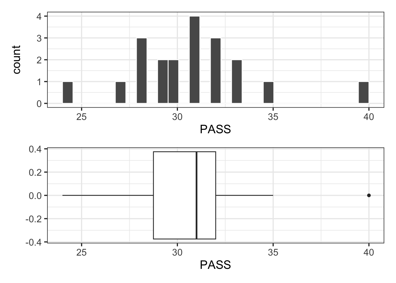
Descriptive statistics:
| n | Min | Max | M | SD |
|---|---|---|---|---|
| 20 | 24 | 40 | 30.7 | 3.31 |
Step 1: Identify the null and alternative hypotheses.
First we need to write the null and alternative hypothesis, which take the form \(H_0 : \mu = \mu_0\) vs \(H_1: \mu \neq \mu_0\). From the research question, we identify the hypothesised value \(\mu_0\) to be 33, hence:
These are written as:
$$H_{0}: \mu = 33$$
$$H_{1}: \mu \neq 33$$
In H_{0} and H_{1} the 0 and 1 within curly braces are written as subscripts. The curly braces delimit what goes in the subscript. The symbol \mu denotes the greek letter “mu” that stands for the population mean (a parameter). The symbol \neq means not equal.
\[H_0: \mu = 33\] \[H_1: \mu \neq 33\]
Step 2: Compute the t-statistic
Next, we compute the t-statistics, which compares the difference between the sample and hypothesised mean (\(\bar{x} - \mu_0\)) to the variation due to random sampling (\(SE_{\bar{x}}\)).
To test the hypothesis, we need to compute the t-statistic,
\[ t = \frac{\bar{x} - \mu_0}{SE_{\bar{x}}} \qquad \text{where} \qquad SE_{\bar{x}} = \frac{s}{\sqrt{n}} \]
# Sample mean
xbar <- stats$M

# Standard error
s <- stats$SD
n <- stats$n
se <- s / sqrt(n)

# Observed t-statistic
tobs <- (xbar - 33) / se
tobs
[1] -3.107272Step 3: Identify the null distribution, i.e. the distribution of the t-statistic assuming the null to be true.
As the sample size is \(n\) = 20, if the null hypothesis is true the t-statistic will follow a t(19) distribution.
Step 4: Compute the critical values for \(\alpha = 0.05\)
As the alternative hypothesis is two-sided (or two-tailed), we have two critical values \(\pm t^*\) that jointly cut an area of 0.05 beyond them. That area must be equally split in both tails, so 0.025 to the left and 0.025 to the right
Hence:
- \(-t^*\) = -2.093024
- \(+t^*\) = +2.093024
Step 5: Make a decision
Compare the observe statistic to the critical values:
tobs[1] -3.107272tstar[1] -2.093024 2.093024Is the observed t-statistic within the critical values (hence we do not reject) or beyond (hence we reject)?
tobs <= tstar[1][1] TRUEtobs >= tstar[2][1] FALSEUsing the critical-value method, we compare the observed t-statistic, -3.11, with the critical values for the appropriate significance level, -2.09 and 2.09. As -3.11 is not within the two critical values, we reject \(H_0\). In fact, -3.11 is smaller than the lower critical value -2.09.
A potential way to report the t-test results:
Example hypothesis test write-up
At the 5% significance level, the sample data provide significant evidence against the null hypothesis and in favour of the alternative one that the mean procrastination score of Edinburgh University students is different from the Solomon & Rothblum reported average of 33: \(t(19) = -3.11, p < .05\), two-sided.
Important: Difference between \(t\) and \(\pm t^*\)
Note the difference between \(\pm t^*\) and the t-statistic \(t\):
The quantiles or critical values are \(-t^*\) and \(+t^*\). These are computed with
qt(..., df = ...). In the quantiles, the superscript \(*\) is not a multiplication sign!The t-statistic \(t = \frac{\bar{x} - \mu_0}{s / \sqrt{n}}\) computes how many standard errors away from the hypothesised value the sample mean is.
4 Student Glossary
To conclude the lab, add the new functions to the glossary of R functions.
| Function | Use and package |
|---|---|
geom_histogram |
? |
geom_boxplot |
? |
summarise |
? |
n() |
? |
mean |
? |
sd |
? |
abs |
? |
qt |
? |
Footnotes
Hint: Ask last week’s driver for the Rmd file, they should share it with the group via email or Teams. To download the file from the server, go to the RStudio Files pane, tick the box next to the Rmd file, and select More > Export.↩︎
-
Hint: Identify the hypothesised value of the mean, \(\mu_0\), and replace that value in the following equations:
\[H_{0} : \mu = \mu_{0}\] \[H_{1} : \mu \neq \mu_{0}\]
The equations can be written with the following code, where the text within curly braces after an underscore is rendered as a subscript:
↩︎$$ H_{0} : \mu = \mu_{0} $$ $$ H_{1} : \mu \neq \mu_{0} $$ -
Hint: Use the following formula for the t-statistic:
\[t = \frac{\bar{x} - \mu_0}{SE_{\bar{x}}} \qquad \text{where} \qquad SE_{\bar{x}} = \frac{s}{\sqrt{n}}\]
In the above:
- \(\bar{x}\) is the sample mean
- \(\mu_0\) is the hypothesised value for the population mean
- \(s\) is the sample standard deviation
- \(n\) is the sample size
Hint: the t-statistic follows a \(t(n-1)\) distribution where \(n-1\) is the degrees of freedom.
The question asks you: what are the degrees of freedom to use in the t distribution?↩︎