| Variable | Description |
|---|---|
| type | College Type: −1 = Not reported; 1 = Public; 2 = Private for-profit; 3 = Private not-for-profit (no religious affiliation); 4 = Private not-for-profit (religious affiliation) |
| region | Region: 0 = US Service schools; 1 = New England; 2 = Mid East; 3 = Great Lakes; 4 = Plains; 5 = Southeast; 6 = Southwest; 7 = Rocky Mountains; 8 = Far West; 9 = Outlying areas |
| gradrate | Graduation Rate – All |
| gradratem | Graduation Rate – Men |
| gradratew | Graduation Rate – Women |
Errors, Power, Effect size, Assumptions
Semester 2 - Week 5
Submission of Formative Report C (PDF file only)
You are required to submit a PDF file by 12 noon on Friday the 17th of February 2023 via Learn. One person needs to submit on behalf of your group.
No extensions allowed. As this is group-based work, no extensions are possible.
-
The report should be at most 6 pages long. At the end of the report, you are allowed two appendices which don’t count towards the page limit.
- Appendix A will contain any tables or figures which you cannot fit in the page limit (no text allowed).
- Appendix B will contain the code to reproduce the report results.
Excluding Appendix B, the report should only include text, figures or tables. It should not include any reference to R code or functions, but be written for a generic reader who is only assumed to have a basic statistical understanding without any R knowledge. You should also avoid any R code output or printout in the PDF file.
The report title should be “Formative Report C (Group 0.A)”. Replace Group 0.A to be your group name.
-
In the author section of the PDF file write the exam number of each person within the group. The exam number starts with the letter B and can be found on your student ID card.
- For example: B000001, B000002, B000003, B000004
You will receive formative feedback on your submission during Flexible Learning Week (next week). Please keep going to the labs next week in order to receive feedback.
1 Tasks
The data dataset-ipeds-2012-subset2, available at https://uoepsy.github.io/data/dataset-ipeds-2012-subset2.csv, is a subset of data derived from the Integrated Postsecondary Education Data System (IPEDS) at the National Center for Education Statistics, 2012. The data were collected for a random sample from all colleges and universities in the United States in that year. The variables include:
In formative report C, you will investigate the mean graduation rate for female students at colleges and universities in the United States. Specifically, you are asked to perform the following tasks, each related to a week of teaching in this course.
This week you will only focus on task C5.
C1) Read the data into R, describe the variable of interest both visually and numerically, and provide a 95% CI for the mean graduation rate of female students at colleges and universities in the United States.
C2) At the 5% significance level and using the p-value method, test whether the mean graduation rate for female students at colleges and universities in the United States is significantly different from a rate of 50 percent.
C3) At the 5% significance level and using the critical value method, test whether the mean graduation rate for female students at colleges and universities in the United States is significantly different from a rate of 50 percent.
C4) Tidy up your report so far, making sure to have 3 sections: introduction, analysis and discussion.
This week’s task
C5) Compute and report the effect size, check if the assumptions underlying the t-test are violated.
2 C5 sub-tasks
In this section you will find some guided sub-steps you may want to consider to complete task C5.
Tip
To see the hints, hover your cursor on the superscript numbers.
- Reopen last week’s Rmd file, as you will continue last week’s work and build on it.1
- Compute an effect size for the graduation rate of female students.2
Add a write-up of the effect size computed above to your report. In other words, after reporting whether the t-test results are statistically significant, are your results also of practical significance (i.e. important)?
Check and report whether the t-test assumptions are satisfied.3
Add a write-up of the assumptions checks to your report.
Knit the report to PDF and submit it via LEARN.
3 Worked Example
The R code is visible for instructional purposes only, but it should not be visible in a PDF report. No R code or output should be visible in a report, only text, figures, and tables.
R code
library(tidyverse)
library(patchwork)
library(kableExtra)

pass_scores <- read_csv("https://uoepsy.github.io/data/pass_scores.csv")
dim(pass_scores)
head(pass_scores)
glimpse(pass_scores)

summary(pass_scores)

plt_hist <- ggplot(pass_scores, aes(x = PASS)) +
    geom_histogram(color = 'white') +
    labs(x = "PASS scores", title = "(a) Histogram")

plt_box <- ggplot(pass_scores, aes(x = PASS)) +
    geom_boxplot() +
    labs(x = "PASS scores", title = "(b) Boxplot")

plt_hist / plt_box
stats <- pass_scores %>%
summarise(n = n(),
Min = min(PASS),
Max = max(PASS),
M = mean(PASS),
SD = sd(PASS))
kbl(stats, booktabs = TRUE, digits = 2,
caption = "Descriptive statistics for PASS scores")
# Confidence interval
xbar <- stats$M
s <- stats$SD
n <- stats$n
se <- s / sqrt(n)
tstar <- qt(c(0.025, 0.975), df = n - 1)
xbar + tstar * se
# observed t-statistic
tobs <- (xbar - 33) / se
tobs
# p-value method
pvalue <- 2 * pt(abs(tobs), df = n - 1, lower.tail = FALSE)
pvalue
# critical values method
tstar
tobs
# effect size
D <- (xbar - 33) / s
D
# assumptions checks
dim(pass_scores)
plt_dens <- ggplot(pass_scores, aes(x = PASS)) +
geom_density() +
labs(x = "PASS scores",
title = "(a) Density plot")
plt_qq <- ggplot(pass_scores, aes(sample = PASS)) +
geom_qq() +
geom_qq_line() +
labs(x = "Theoretical quantiles",
y = "Sample quantiles",
title = "(b) QQ-plot")
plt_dens | plt_qqshapiro.test(pass_scores$PASS)
Introduction
A random sample of 20 students from the University of Edinburgh completed a questionnaire measuring their total endorsement of procrastination. The data, available from https://uoepsy.github.io/data/pass_scores.csv, were used to estimate the average procrastination score of all Edinburgh University students, as well as testing whether the mean procrastination score differed from the Solomon & Rothblum reported average of 33 at the 5% significance level. The recorded variables include a subject identifier (sid, categorical), the school each belongs to (school, categorical), and the total score on the Procrastination Assessment Scale for Students (PASS, numeric). The data did not include any impossible values for the PASS scores, as they were all within the possible range of 0 – 90. To answer the questions of interest, we only focused on the total PASS score variable.
Analysis
Throughout the report we used a significance level \(\alpha\) of 5%.
The distribution of PASS scores, as shown in Figure 1(a), is roughly bell shaped and does not have any impossible values. The outlier (40) depicted in the boxplot shown in Figure 1(b) is well within the range of plausible values for the PASS scale (0–90) and as such was not removed for the analysis.
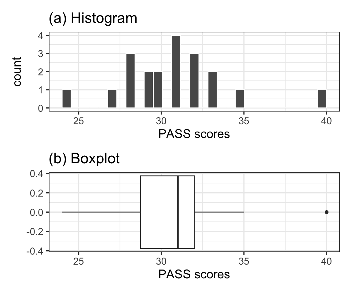
| n | Min | Max | M | SD |
|---|---|---|---|---|
| 20 | 24 | 40 | 30.7 | 3.31 |
Table 1 displays summary statistics for the PASS scores in the sample of Edinburgh University students. From the sample data we obtain an average procrastination score of \(M = 30.7\), 95% CI [29.15, 32.25]. Hence, we are 95% confident that a Edinburgh University student will have a procrastination score between 29.15 and 32.25, which is between 0.75 and 3.85 lower than the average score of 33 reported by Solomon & Rothblum.
To investigate whether the mean PASS scores of all Edinburgh University students, \(\mu\) say, differs from the Solomon & Rothblum reported average of 33, we performed a one sample t-test of \(H_0 : \mu = 33\) against \(H_1 : \mu \neq 33\). The sample data provided very strong evidence against the null hypothesis and in favour of the alternative one that the mean procrastination score of Edinburgh University students is significantly different from the Solomon & Rothblum reported average of 33: \(t(19) = -3.11, p = .006\), two-sided. The size of the effect was also found to be medium to large \((D = -0.69)\).
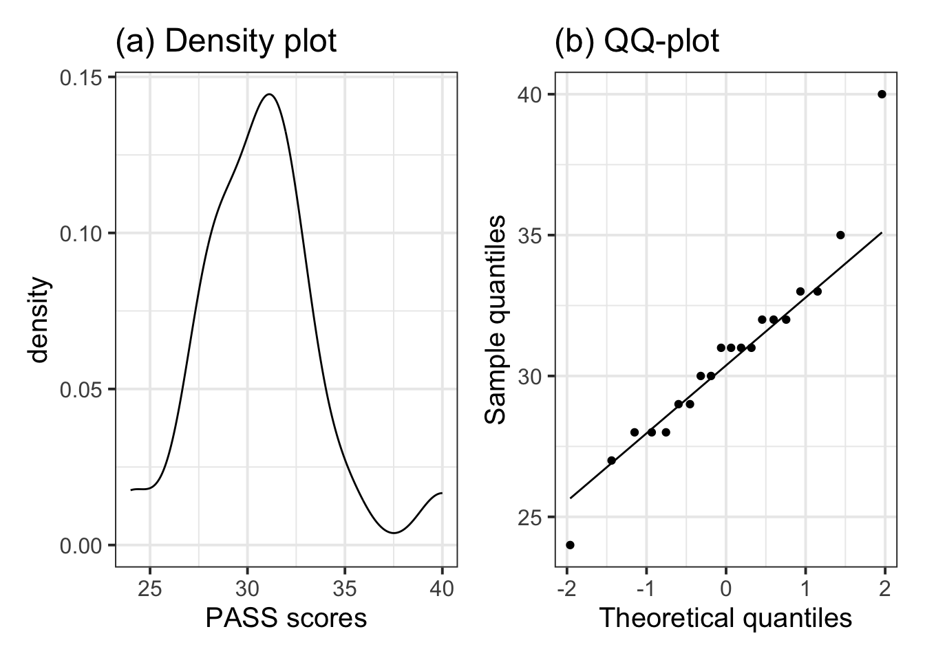
The sample data did not show violations of the assumptions required for the t-test results to be valid. Specifically, the data were collected on a random sample of students from Edinburgh University, hence independence was met. Figure 2(a) shows that the distribution of PASS scores is roughly bell-shaped, with a single mode and as such does not raise any concerns of violations of normality. Similarly, the QQ-plot in Figure 2(b) shows agreement between the sample and theoretical quantiles, as they almost all fall on the line. We also performed a Shapiro-Wilk test against the null hypothesis of normality of the population data: \(W = 0.94\), \(p = .20\). The sample data did not provide sufficient evidence at the 5% level to reject the null hypothesis that the population data follow a normal distribution.
Discussion
Data including the Procrastination Assessment Scale for Students (PASS) scores for a random sample of 20 students at Edinburgh University were used to estimate the average procrastination score for a student of that university. In addition, the data were used to test whether there is a significant difference between that average score and the Solomon & Rothblum reported average of 33.
The data provided very strong evidence that the mean procrastination score of Edinburgh University students differs from 33. Furthermore, the data indicate that a Edinburgh University student tends to have a mean procrastination score between 29.15 and 32.35, which is 0.75 and 3.85 lower than the Solomon & Rothblum reported average of 33.
What is missing from this instructional example:
- Appendix A
- Appendix B
Footnotes
Hint: Ask last week’s driver for the Rmd file, they should share it with the group via email or Teams. To download the file from the server, go to the RStudio Files pane, tick the box next to the Rmd file, and select More > Export.↩︎
-
Hint: Cohen’s \(D\) for a one sample t-test is given by
\[D = \frac{\bar{x} - \mu_0}{s}\]
where \(\bar{x}\) is the sample mean, \(\mu_0\) is the value for the population mean that we hypothesised in the null hypothesis (50), and \(s\) is the sample standard deviation.↩︎
-
Hint: Recall that, for the t-test results to be valid, conditions (1) and (2) below need to be met:
- The data need to come from a random sample of the population
- Either one of these holds:
- The population follows a normal distribution (irrespectively of the sample size)
- The sample size is large enough, \(n \geq 30\) as a guideline.
For (1), this is known from the study design description. For (2) some of these functions may be useful:
dim,nrow,geom_qq,geom_qq_line,shapiro.test.↩︎