W9 Exercises: EFA

Conduct Problems

Data: Conduct Problems

A researcher is developing a new brief measure of Conduct Problems. She has collected data from n=450 adolescents on 10 items, which cover the following behaviours:

1. Breaking curfew
2. Vandalism
3. Skipping school
4. Bullying
5. Spreading malicious rumours
6. Fighting
7. Lying
8. Using a weapon
9. Stealing
10. Threatening others

Our task is to use the dimension reduction techniques we learned about in the lecture to help inform how to organise the items she has developed into subscales.

The data can be found at https://uoepsy.github.io/data/conduct_probs_scale.csv

Question 1

Read in the dataset.
Create a correlation matrix for the items, and inspect the items to check their suitability for exploratory factor analysis

Hints

Take a look at Reading 9# Initial Checks.

cpdata <- read.csv("https://uoepsy.github.io/data/conduct_probs_scale.csv")
# discard the first column
cpdata <- cpdata[,-1]

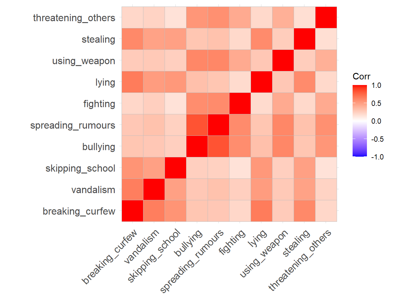
Here’s a correlation matrix. There’s no obvious blocks of items here, but we can see that there are some fairly high correlations, as well as some weaker ones. All are positive.

library(ggcorrplot)
ggcorrplot(cor(cpdata))

The Bartlett’s test comes out with a p-value of 0 (which isn’t possible, but it’s been rounded for some reason). This suggests that we reject the null of this test (that our correlation matrix is proportional to the identity matrix). This is good. It basically means “we have some non-zero correlations”!

library(psych)
cortest.bartlett(cor(cpdata), n=450)

$chisq
[1] 2238

$p.value
[1] 0

$df
[1] 45

The overall sampling adequacy is 0.87, which is pretty good! (or rather, which is ‘meritorious’!). MSA for all items is >.8

KMO(cpdata)  

Kaiser-Meyer-Olkin factor adequacy
Call: KMO(r = cpdata)
Overall MSA =  0.87
MSA for each item = 
   breaking_curfew          vandalism    skipping_school           bullying 
              0.84               0.88               0.92               0.82 
 spreading_rumours           fighting              lying       using_weapon 
              0.81               0.94               0.88               0.95 
          stealing threatening_others 
              0.90               0.94 

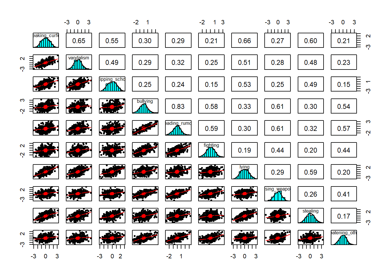
Finally, all the relationships here look fairly linear:

pairs.panels(cpdata)

Question 2

How many dimensions should be retained?

This question can be answered in the same way as we did for PCA - use a scree plot, parallel analysis, and MAP test to guide you.

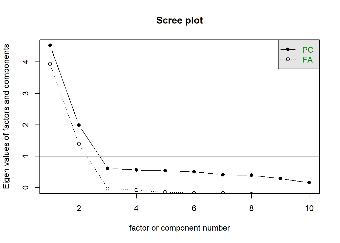
The scree plot shows a kink at 3, which suggests retaining 2 components.

scree(cpdata)

The MAP suggests retaining 2 factors. I’m just extracting the actual map values here to save having to show all the other output. We can see that the 2nd entry is the smallest:

VSS(cpdata, plot = FALSE, n = ncol(cpdata))$map

 [1] 0.1058 0.0338 0.0576 0.1035 0.1494 0.2520 0.3974 0.4552 1.0000     NA

Parallel analysis suggests 2 factors as well:

fa.parallel(cpdata, fa = "both")

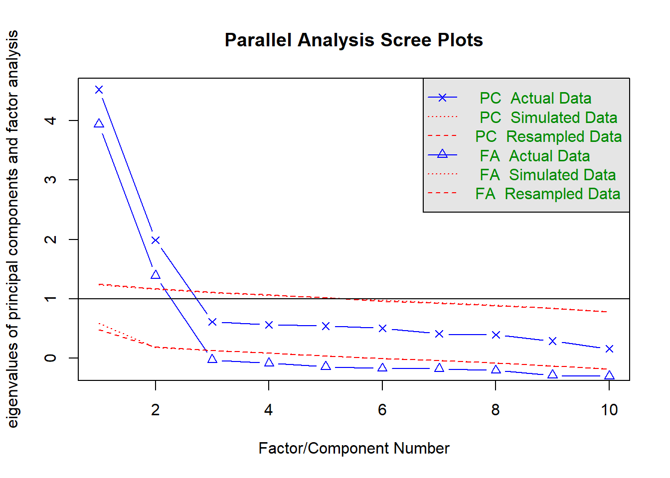
Parallel analysis suggests that the number of factors =  2  and the number of components =  2 

Again, a quite clear picture that 2 factors is preferred:

guides	suggestion
Scree	2
MAP	2
Parallel Analysis	2

Question 3

Use the function fa() from the psych package to conduct and EFA to extract 2 factors (this is what we suggest based on the various tests above, but you might feel differently - the ideal number of factors is subjective!). Use a suitable rotation (rotate = ?) and extraction method (fm = ?).

Hints

Would you expect factors to be correlated? If so, you’ll want an oblique rotation.
See R9#doing-an-efa.

For example, you could choose an oblimin rotation to allow factors to correlate. Let’s use MLE as the estimator.

conduct_efa <- fa(cpdata, nfactors=2, rotate='oblimin', fm="ml")

Question 4

Inspect your solution. Make sure to look at and think about the loadings, the variance accounted for, and the factor correlations (if estimated).

Hints

Just printing an fa object:

myfa <- fa(data, ..... )
myfa

Will give you lots and lots of information.
You can extract individual parts using:

• myfa$loadings for the loadings
• myfa$Vaccounted for the variance accounted for by each factor
• myfa$Phi for the factor correlation matrix

You can find a quick guide to reading the fa output here: efa_output.pdf.

Things look pretty good here. Each item has a clear primary loading on to one of the factors, and the complexity for all items is 1 (meaning they’re clearly link to just one of the factors). The h2 column is showing that the 2 factor solution is explaining 39%+ of the variance in each item. Both factors are well determined, having a at least 3 salient loadings.

The 2 factors together explain 57% of the variance in the data - both factors explain a similar amount (29% for factor 1, 28% for factor 2).

We can also see that there is a moderate correlation between the two factors. Use of an oblique rotation was appropriate - if the correlation had been very weak, then it might not have differed much from if we used an orthogonal rotation.

conduct_efa

Factor Analysis using method =  ml
Call: fa(r = cpdata, nfactors = 2, rotate = "oblimin", fm = "ml")
Standardized loadings (pattern matrix) based upon correlation matrix
                     ML1   ML2   h2   u2 com
breaking_curfew    -0.05  0.88 0.74 0.26   1
vandalism           0.05  0.69 0.51 0.49   1
skipping_school    -0.01  0.67 0.44 0.56   1
bullying            0.90  0.00 0.81 0.19   1
spreading_rumours   0.93 -0.02 0.85 0.15   1
fighting            0.65 -0.02 0.42 0.58   1
lying               0.02  0.77 0.60 0.40   1
using_weapon        0.63  0.09 0.45 0.55   1
stealing            0.04  0.70 0.51 0.49   1
threatening_others  0.62 -0.01 0.38 0.62   1

                       ML1  ML2
SS loadings           2.91 2.80
Proportion Var        0.29 0.28
Cumulative Var        0.29 0.57
Proportion Explained  0.51 0.49
Cumulative Proportion 0.51 1.00

 With factor correlations of 
     ML1  ML2
ML1 1.00 0.43
ML2 0.43 1.00

Mean item complexity =  1

Question 5

Look back to the description of the items, and suggest a name for your factors based on the patterns of loadings.

Hints

To sort the loadings, you can use

print(myfa$loadings, sort = TRUE)

You can inspect the loadings using:

print(conduct_efa$loadings, sort=TRUE)

Loadings:
                   ML1    ML2   
bullying            0.899       
spreading_rumours   0.931       
fighting            0.653       
using_weapon        0.629       
threatening_others  0.621       
breaking_curfew            0.878
vandalism                  0.694
skipping_school            0.671
lying                      0.767
stealing                   0.696

                 ML1   ML2
SS loadings    2.890 2.782
Proportion Var 0.289 0.278
Cumulative Var 0.289 0.567

We can see that, ordered like this, we have five items that have high loadings for one factor and another five items that have high loadings for the other.

The five items for factor 2 all have in common that they are non-aggressive forms of conduct problems. The five items for factor 1 are all more aggressive behaviours. We could, therefore, label our factors: ‘aggressive’ and ‘non-aggressive’ conduct problems.

Question 6

Compare three different solutions:

1. your current solution from the previous questions
2. one where you fit 1 more factor
3. one where you fit 1 fewer factors

Which one looks best?

Hints

We’re looking here to assess:

• how much variance is accounted for by each solution
• do all factors load on 3+ items at a salient level?
  
• do all items have at least one loading at a salient level?
• are there any “Heywood cases” (communalities or standardised loadings that are >1)?
• should we perhaps remove some of the more complex items?
• is the factor structure (items that load on to each factor) coherent, and does it make theoretical sense?

The 1-factor model explains 37% of the variance (as opposed to the 57% explained by the 2 factor solution), and all items load fairly high on the factor. The downside here is that we’re not discerning between different types of conduct problems that we did in the 2 factor solution.

conduct_1 <- fa(cpdata, nfactors=1, fm="ml")
conduct_1

Factor Analysis using method =  ml
Call: fa(r = cpdata, nfactors = 1, fm = "ml")
Standardized loadings (pattern matrix) based upon correlation matrix
                    ML1   h2   u2 com
breaking_curfew    0.42 0.18 0.82   1
vandalism          0.42 0.18 0.82   1
skipping_school    0.35 0.13 0.87   1
bullying           0.89 0.79 0.21   1
spreading_rumours  0.90 0.81 0.19   1
fighting           0.64 0.41 0.59   1
lying              0.43 0.18 0.82   1
using_weapon       0.68 0.46 0.54   1
stealing           0.42 0.17 0.83   1
threatening_others 0.61 0.38 0.62   1

                ML1
SS loadings    3.69
Proportion Var 0.37

Mean item complexity =  1
Test of the hypothesis that 1 factor is sufficient.

df null model =  45  with the objective function =  5.03 with Chi Square =  2238
df of  the model are 35  and the objective function was  1.78 

The root mean square of the residuals (RMSR) is  0.19 
The df corrected root mean square of the residuals is  0.22 

The harmonic n.obs is  450 with the empirical chi square  1465  with prob <  1.9e-285 
The total n.obs was  450  with Likelihood Chi Square =  789  with prob <  3.4e-143 

Tucker Lewis Index of factoring reliability =  0.557
RMSEA index =  0.219  and the 90 % confidence intervals are  0.206 0.232
BIC =  575
Fit based upon off diagonal values = 0.8
Measures of factor score adequacy             
                                                   ML1
Correlation of (regression) scores with factors   0.96
Multiple R square of scores with factors          0.92
Minimum correlation of possible factor scores     0.84

The 3-factor model explains 60% of the variance (only 3% more than the 2-factor model). Notably, the third factor is not very clearly defined - it only has 1 salient loading (possibly 2 if we consider the 0.3 to be salient, but that item is primarily loaded on the 2nd factor).

conduct_3 <- fa(cpdata, nfactors=3, rotate='oblimin', fm="ml")
conduct_3

Factor Analysis using method =  ml
Call: fa(r = cpdata, nfactors = 3, rotate = "oblimin", fm = "ml")
Standardized loadings (pattern matrix) based upon correlation matrix
                     ML1   ML2   ML3   h2   u2 com
breaking_curfew    -0.02  0.61  0.31 0.71 0.29 1.5
vandalism           0.06  0.12  0.74 0.72 0.28 1.1
skipping_school     0.00  0.56  0.14 0.44 0.56 1.1
bullying            0.90  0.09 -0.10 0.82 0.18 1.0
spreading_rumours   0.92 -0.02  0.03 0.85 0.15 1.0
fighting            0.65 -0.13  0.14 0.43 0.57 1.2
lying               0.02  0.85 -0.06 0.67 0.33 1.0
using_weapon        0.63  0.08  0.02 0.45 0.55 1.0
stealing            0.06  0.69  0.02 0.53 0.47 1.0
threatening_others  0.62 -0.08  0.09 0.39 0.61 1.1

                       ML1  ML2  ML3
SS loadings           2.93 2.14 0.94
Proportion Var        0.29 0.21 0.09
Cumulative Var        0.29 0.51 0.60
Proportion Explained  0.49 0.36 0.16
Cumulative Proportion 0.49 0.84 1.00

 With factor correlations of 
     ML1  ML2  ML3
ML1 1.00 0.39 0.32
ML2 0.39 1.00 0.68
ML3 0.32 0.68 1.00

Mean item complexity =  1.1
Test of the hypothesis that 3 factors are sufficient.

df null model =  45  with the objective function =  5.03 with Chi Square =  2238
df of  the model are 18  and the objective function was  0.02 

The root mean square of the residuals (RMSR) is  0.01 
The df corrected root mean square of the residuals is  0.02 

The harmonic n.obs is  450 with the empirical chi square  3.98  with prob <  1 
The total n.obs was  450  with Likelihood Chi Square =  10.5  with prob <  0.91 

Tucker Lewis Index of factoring reliability =  1.01
RMSEA index =  0  and the 90 % confidence intervals are  0 0.016
BIC =  -99.5
Fit based upon off diagonal values = 1
Measures of factor score adequacy             
                                                   ML1  ML2  ML3
Correlation of (regression) scores with factors   0.96 0.93 0.88
Multiple R square of scores with factors          0.93 0.86 0.77
Minimum correlation of possible factor scores     0.85 0.72 0.53

Question 7

Write a brief paragraph or two that summarises your method and the results from your chosen optimal factor structure for the 10 conduct problems.

Hints

Write about the process that led you to the number of factors. Discuss the patterns of loadings and provide definitions of the factors.

The main principles governing the reporting of statistical results are transparency and reproducibility (i.e., someone should be able to reproduce your analysis based on your description).

An example summary would be:

First, the data were checked for their suitability for factor analysis. Normality was checked using visual inspection of histograms, linearity was checked through the inspection of the linear and lowess lines for the pairwise relations of the variables, and factorability was confirmed using a KMO test, which yielded an overall KMO of \(.87\) with no variable KMOs \(<.50\). An exploratory factor analysis was conducted to inform the structure of a new conduct problems test. Inspection of a scree plot alongside parallel analysis (using principal components analysis; PA-PCA) and the MAP test were used to guide the number of factors to retain. All three methods suggested retaining two factors; however, a one-factor and three-factor solution were inspected to confirm that the two-factor solution was optimal from a substantive and practical perspective, e.g., that it neither blurred important factor distinctions nor included a minor factor that would be better combined with the other in a one-factor solution. These factor analyses were conducted using maximum likelihood estimation and (for the two- and three-factor solutions) an oblimin rotation, because it was expected that the factors would correlate. Inspection of the factor loadings and correlations reinforced that the two-factor solution was optimal: both factors were well-determined, including 5 loadings \(>|0.3|\) and the one-factor model blurred the distinction between different forms of conduct problems. The factor loadings are provided in Table 1¹. Based on the pattern of factor loadings, the two factors were labelled ‘aggressive conduct problems’ and ‘non-aggressive conduct problems’. These factors had a correlation of \(r=.43\). Overall, they accounted for 57% of the variance in the items, suggesting that a two-factor solution effectively summarised the variation in the items.

Table 1: Factor Loadings

	ML1	ML2
spreading_rumours	0.93
bullying	0.90
fighting	0.65
using_weapon	0.63
threatening_others	0.62
vandalism		0.88
stealing		0.77
lying		0.70
skipping_school		0.69
breaking_curfew		0.67

Dimensions of Apathy

Dataset: radakovic_das.csv

Apathy is lack of motivation towards goal-directed behaviours. It is pervasive in a majority of psychiatric and neurological diseases, and impacts everyday life. Traditionally, apathy has been measured as a one-dimensional construct, it may be that multiple different types of demotivation provides a better explanation.

We have data on 250 people who have responded to 24 questions about apathy, that can be accessed at https://uoepsy.github.io/data/radakovic_das.csv. Information on the items can be seen in the table below.

DAS Dictionary

All items are measured on a 6-point Likert scale of Always (0), Almost Always (1), Often (2), Occasionally (3), Hardly Ever (4), and Never (5). Certain items (indicated in the table below with a - direction) are reverse scored to ensure that higher scores indicate greater levels of apathy.

item	direction	question
1	+	I need a bit of encouragement to get things started
2	-	I contact my friends
3	-	I express my emotions
4	-	I think of new things to do during the day
5	-	I am concerned about how my family feel
6	+	I find myself staring in to space
7	-	Before I do something I think about how others would feel about it
8	-	I plan my days activities in advance
9	-	When I receive bad news I feel bad about it
10	-	I am unable to focus on a task until it is finished
11	+	I lack motivation
12	+	I struggle to empathise with other people
13	-	I set goals for myself
14	-	I try new things
15	+	I am unconcerned about how others feel about my behaviour
16	-	I act on things I have thought about during the day
17	+	When doing a demanding task, I have difficulty working out what I have to do
18	-	I keep myself busy
19	+	I get easily confused when doing several things at once
20	-	I become emotional easily when watching something happy or sad on TV
21	+	I find it difficult to keep my mind on things
22	-	I am spontaneous
23	+	I am easily distracted
24	+	I feel indifferent to what is going on around me

Question 8

Here is some code that does the following:

• reads in the data
• renames the variables as “q1”, “q2”, “q3”, … and so on
• recodes the variables so that instead of words, the responses are coded as numbers

rdas <- read_csv("https://uoepsy.github.io/data/radakovic_das.csv")

names(rdas) <- paste0("q",1:24)

rdas <- rdas |> 
  mutate(across(q1:q24, ~case_match(.,
    "Always" ~ 0,
    "Almost Always" ~ 1,
    "Often" ~ 2,
    "Occasionally" ~ 3,
    "Hardly Ever" ~ 4,
    "Never" ~ 5
  )))

What number of underlying dimensions best explain the variability in the questionnaire?

Check the suitability of the items before conducting exploratory factor analysis to address this question. Decide on an optimal factor solution and provide a theoretical name for each factor. We’re not doing scale development here, so ideally we don’t want to get rid of items.

Once you’ve tried, have a look at this paper by Radakovic & Abrahams that is essentially what you’ve just done! (the data isn’t the same, ours is fake!).

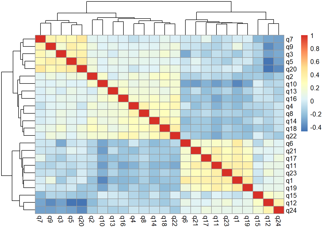
Here are all the item correlations:

library(pheatmap)
cor(rdas, use = "complete") |> pheatmap()

everything is pretty high in the KMO factor adequacy:

KMO(rdas)

Kaiser-Meyer-Olkin factor adequacy
Call: KMO(r = rdas)
Overall MSA =  0.82
MSA for each item = 
  q1   q2   q3   q4   q5   q6   q7   q8   q9  q10  q11  q12  q13  q14  q15  q16 
0.82 0.81 0.77 0.80 0.83 0.75 0.77 0.80 0.76 0.88 0.88 0.83 0.78 0.87 0.73 0.88 
 q17  q18  q19  q20  q21  q22  q23  q24 
0.87 0.84 0.78 0.78 0.88 0.78 0.87 0.87 

How many factors should we consider?

scree(rdas)

vss(rdas, plot = FALSE)

Very Simple Structure
Call: vss(x = rdas, plot = FALSE)
VSS complexity 1 achieves a maximimum of 0.63  with  2  factors
VSS complexity 2 achieves a maximimum of 0.7  with  4  factors

The Velicer MAP achieves a minimum of 0.01  with  2  factors 
BIC achieves a minimum of  -953  with  2  factors
Sample Size adjusted BIC achieves a minimum of  -258  with  3  factors

Statistics by number of factors 
  vss1 vss2    map dof chisq    prob sqresid  fit  RMSEA  BIC SABIC complex
1 0.45 0.00 0.0197 252   714 8.7e-46    24.3 0.45 0.0856 -677   122     1.0
2 0.63 0.67 0.0098 229   312 2.2e-04    14.8 0.67 0.0378 -953  -227     1.1
3 0.56 0.69 0.0107 207   229 1.4e-01    13.0 0.71 0.0202 -914  -258     1.3
4 0.55 0.70 0.0130 186   190 4.0e-01    12.0 0.73 0.0086 -837  -247     1.4
5 0.53 0.68 0.0155 166   159 6.3e-01    11.1 0.75 0.0000 -757  -231     1.6
6 0.55 0.67 0.0188 147   131 8.3e-01    10.3 0.77 0.0000 -681  -215     1.9
7 0.54 0.67 0.0224 129   107 9.2e-01     9.7 0.78 0.0000 -605  -196     2.0
8 0.54 0.68 0.0267 112    88 9.5e-01     9.2 0.79 0.0000 -530  -175     2.1
  eChisq  SRMR eCRMS eBIC
1   1751 0.113 0.118  360
2    376 0.052 0.057 -889
3    227 0.041 0.047 -916
4    180 0.036 0.044 -847
5    135 0.031 0.040 -781
6    105 0.028 0.038 -707
7     83 0.025 0.036 -629
8     64 0.022 0.034 -554

fa.parallel(rdas)

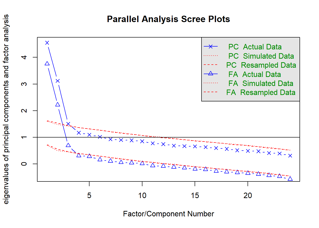
Parallel analysis suggests that the number of factors =  3  and the number of components =  3 

criterion	suggestion
kaiser	2
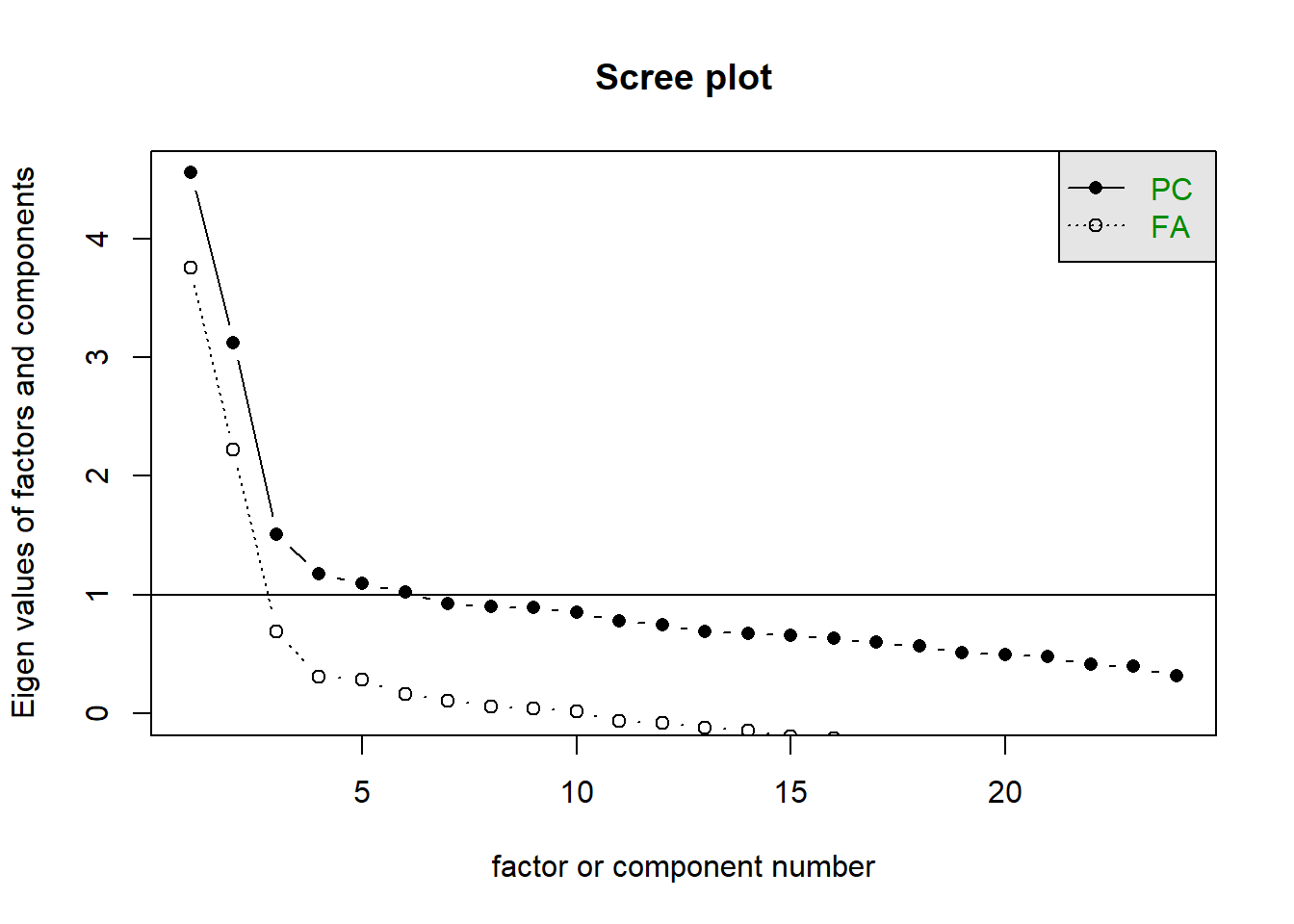
scree plot	3
parallel analysis	3
MAP	2

Seems like we should consider a 2 factor and a 3 factor solution. I reckon any underlying dimensions of apathy are likely to be quite related to one another, so we’ll use an oblique rotation.

apath2 <- fa(rdas, nfactors = 2, rotate = "oblimin", fm = "ml")
apath3 <- fa(rdas, nfactors = 3, rotate = "oblimin", fm = "ml")

The three factor model explains 30% of the variance, but there are various items that seem to load across all 3 factors (q2, q15, q16), and for some of these none of them are ‘salient’ (i.e. above 0.3).

print(apath3$loadings, sort=TRUE)

Loadings:
    ML2    ML1    ML3   
q3   0.528 -0.196       
q5   0.649              
q7   0.581        -0.151
q9   0.511  0.106       
q12 -0.667        -0.110
q20  0.714              
q24 -0.526              
q1          0.812       
q6          0.527       
q10        -0.534       
q4                 0.539
q18  0.100         0.553
q22                0.535
q2   0.162 -0.138  0.249
q8                 0.418
q11         0.450 -0.237
q13        -0.256  0.125
q14                0.440
q15 -0.311 -0.166 -0.165
q16        -0.201  0.307
q17         0.433 -0.125
q19         0.437 -0.135
q21         0.431 -0.124
q23         0.496       

                 ML2   ML1   ML3
SS loadings    2.682 2.459 1.618
Proportion Var 0.112 0.102 0.067
Cumulative Var 0.112 0.214 0.282

The two factor solution explains 26% of the variance, and only one item (q2) is below 0.3 (and only just!).

print(apath2$loadings, sort=TRUE)

Loadings:
    ML1    ML2   
q1   0.697       
q10 -0.553       
q11  0.608       
q17  0.508       
q19  0.514       
q21  0.506       
q23  0.519       
q5          0.648
q7          0.547
q9          0.529
q12        -0.686
q20         0.716
q24        -0.523
q2  -0.298  0.192
q3  -0.117  0.496
q4  -0.387       
q6   0.466       
q8  -0.311       
q13 -0.329       
q14 -0.397       
q15        -0.345
q16 -0.411       
q18 -0.401  0.177
q22 -0.399       

                 ML1   ML2
SS loadings    3.545 2.718
Proportion Var 0.148 0.113
Cumulative Var 0.148 0.261

Hard to decide here. I think I need to know more about “apathy” to make an informed decision about the items.
Radakovic & Abrahams end up with 3 factors:

• “Executive” - this is similar to the second factor (“ML1”) in our 3-factor model
  
• “Emotional” - this is like the first factor (“ML2”) in our 3-factor model
  
• “Initiation” - the third factor (“ML3”) in our 3-factor model

Footnotes

1. You should provide the table of factor loadings. It is conventional to omit factor loadings \(<|0.3|\); however, be sure to ensure that you mention this in a table note.