W10 Exercises: EFA, replicability, reliability

More EFA

Data: petmoods2.csv

A pet food company has conducted a questionnaire on the internet (\(n = 620\)) to examine whether owning a pet influences low mood. They asked 16 questions on a Likert scale (1-7, detailed below) followed by a simple Yes/No question concerning whether the respondent owned a pet.

The researchers don’t really know much about the theory of mood disorders, but they looked at some other questionnaires and copied the questions they saw often appearing. They think that they are likely picking up on multiple different types of “low mood”, so they want do an EFA to examine this. They then want to look at group differences (pet owners vs not pet owners) in the dimensions of low mood.

The data are available at https://uoepsy.github.io/data/petmoods2.csv

QuestionNumber Over the last 2 weeks, how much have you had/have you been...
item1 Little interest or pleasure in doing things?
item2 Feeling down, depressed, or hopeless?
item3 Trouble falling or staying asleep, or sleeping too much?
item4 Feeling tired or having little energy?
item5 Poor appetite or overeating?
item6 Feeling bad about yourself - or that you are a failure or have let yourself or your family down?
item7 Trouble concentrating on things, such as reading the newspaper or watching television?
item8 Moving or speaking so slowly that other people could have noticed? Or the opposite - being so fidgety or restless that you have been moving around a lot more than usual?
item9 A lack of motivation to do anything at all?
item10 Feeling nervous, anxious or on edge?
item11 Not being able to stop or control worrying?
item12 Worrying too much about different things?
item13 Trouble relaxing?
item14 Being so restless that it is hard to sit still?
item15 Becoming easily annoyed or irritable?
item16 Feeling afraid as if something awful might happen?
Question 1

Read in the data, check the suitability for conducting factor analysis, and then examine what underlying dimensions best explain the observed relationships between the 16 mood-related questions in the survey.

library(tidyverse)
library(psych)
petdata <- read_csv("https://uoepsy.github.io/data/petmoods2.csv")
names(petdata)
 [1] "ppt_id"                                                                                                                                                               
 [2] "do_you_own_a_pet"                                                                                                                                                     
 [3] "little_interest_or_pleasure_in_doing_things"                                                                                                                          
 [4] "feeling_down_depressed_or_hopeless"                                                                                                                                   
 [5] "trouble_falling_or_staying_asleep_or_sleeping_too_much"                                                                                                               
 [6] "feeling_tired_or_having_little_energy"                                                                                                                                
 [7] "poor_appetite_or_overeating"                                                                                                                                          
 [8] "feeling_bad_about_yourself_or_that_you_are_a_failure_or_have_let_yourself_or_your_family_down"                                                                        
 [9] "trouble_concentrating_on_things_such_as_reading_the_newspaper_or_watching_television"                                                                                 
[10] "moving_or_speaking_so_slowly_that_other_people_could_have_noticed_or_the_opposite_being_so_fidgety_or_restless_that_you_have_been_moving_around_a_lot_more_than_usual"
[11] "a_lack_of_motivation_to_do_anything_at_all"                                                                                                                           
[12] "feeling_nervous_anxious_or_on_edge"                                                                                                                                   
[13] "not_being_able_to_stop_or_control_worrying"                                                                                                                           
[14] "worrying_too_much_about_different_things"                                                                                                                             
[15] "trouble_relaxing"                                                                                                                                                     
[16] "being_so_restless_that_it_is_hard_to_sit_still"                                                                                                                       
[17] "becoming_easily_annoyed_or_irritable"                                                                                                                                 
[18] "feeling_afraid_as_if_something_awful_might_happen"                                                                                                                    

I’m going to subset out the mood data for now, to make it easier to work with:

moodq <- petdata %>% 
    select(-ppt_id, -do_you_own_a_pet)

And then rename the variables:

names(moodq) <- paste0("item", 1:ncol(moodq))
head(moodq)
# A tibble: 6 × 16
  item1 item2 item3 item4 item5 item6 item7 item8 item9 item10 item11 item12
  <dbl> <dbl> <dbl> <dbl> <dbl> <dbl> <dbl> <dbl> <dbl>  <dbl>  <dbl>  <dbl>
1     6     4     4     5     5     5     4     3     2      4      6      4
2     3     5     5     6     3     5     3     5     3      5      4      3
3     6     7     7     6     5     4     7     6     6      5      3      6
4     5     4     4     4     4     2     5     2     5      3      6      2
5     6     6     5     5     5     4     7     2     2      6      6      3
6     4     5     5     5     3     4     5     3     3      5      4      4
# ℹ 4 more variables: item13 <dbl>, item14 <dbl>, item15 <dbl>, item16 <dbl>

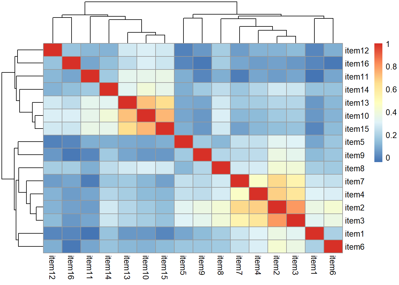
pheatmap::pheatmap(cor(moodq))

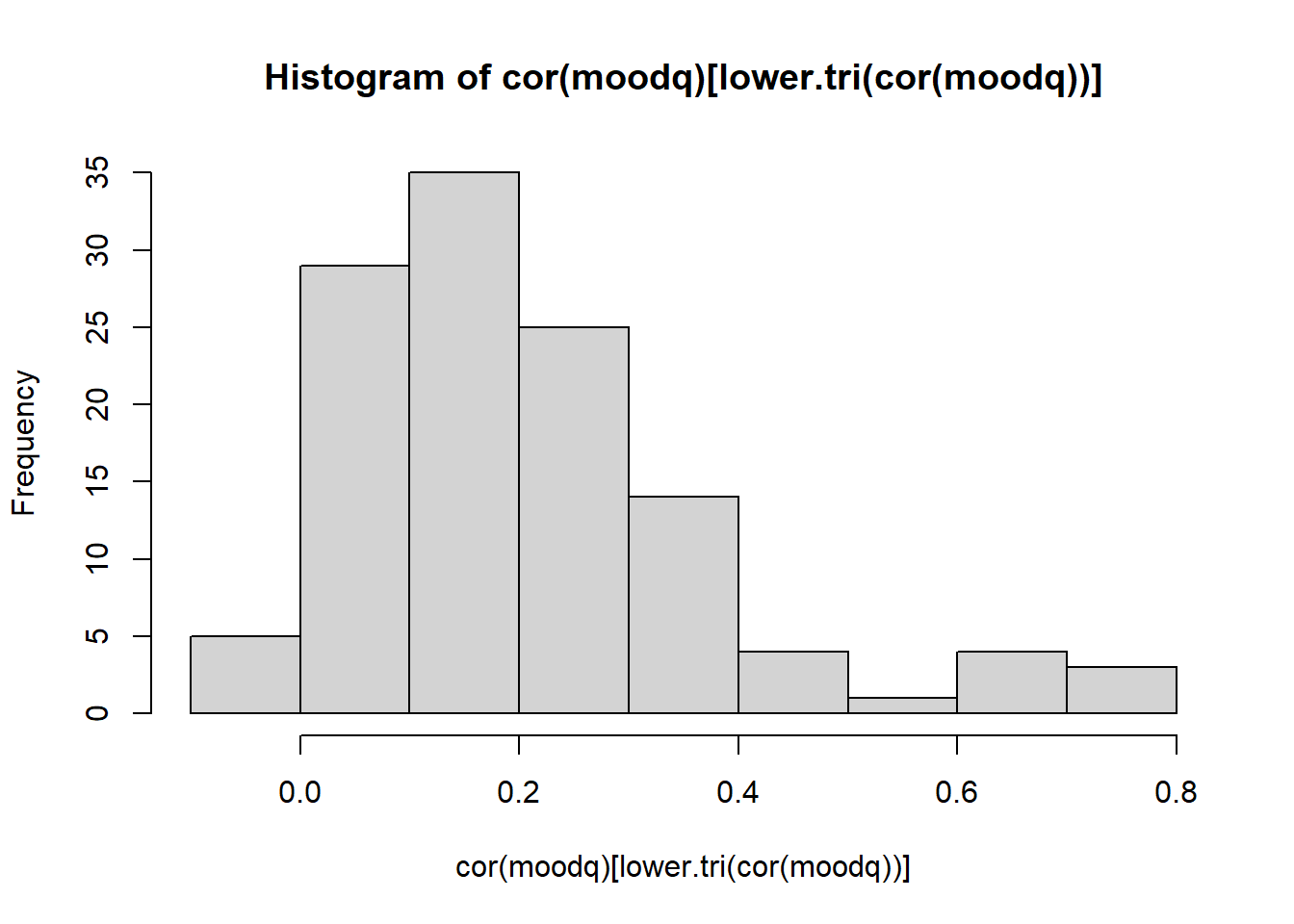
cor(moodq)[lower.tri(cor(moodq))] |> hist()

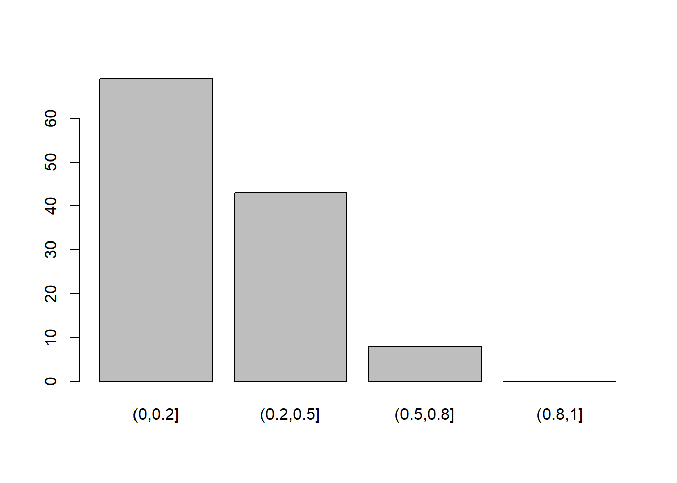
cut(abs(cor(moodq)[lower.tri(cor(moodq))]),c(0,.2,.5,.8,1)) |>
  table() |>
  barplot()

KMO(moodq)
Kaiser-Meyer-Olkin factor adequacy
Call: KMO(r = moodq)
Overall MSA =  0.87
MSA for each item = 
 item1  item2  item3  item4  item5  item6  item7  item8  item9 item10 item11 
  0.93   0.80   0.88   0.91   0.92   0.92   0.88   0.94   0.91   0.80   0.90 
item12 item13 item14 item15 item16 
  0.91   0.86   0.93   0.84   0.87 

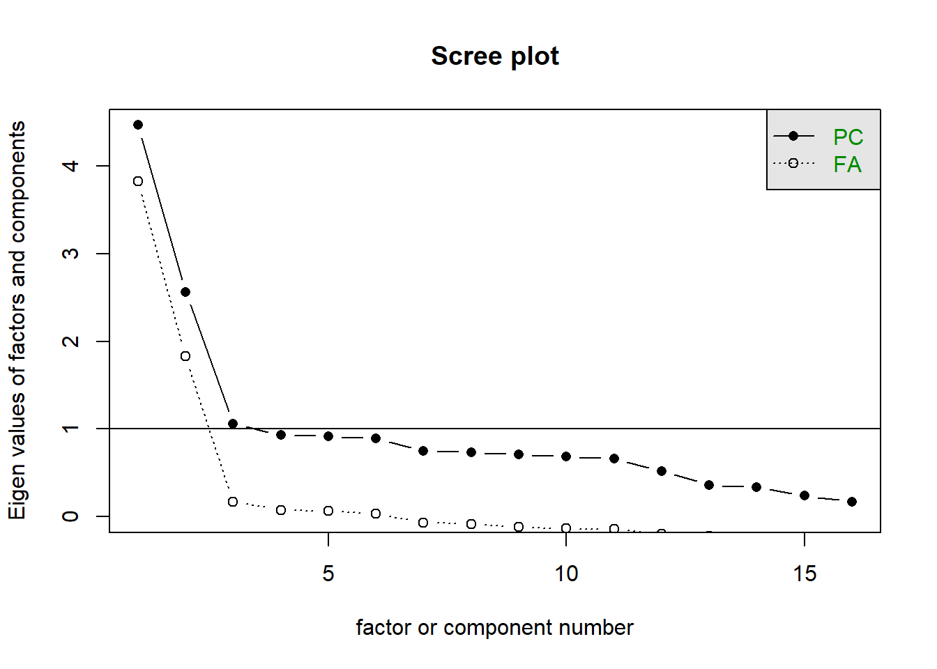
scree(moodq)

VSS(moodq, plot=FALSE)$map
[1] 0.0484 0.0123 0.0189 0.0278 0.0385 0.0520 0.0741 0.1044
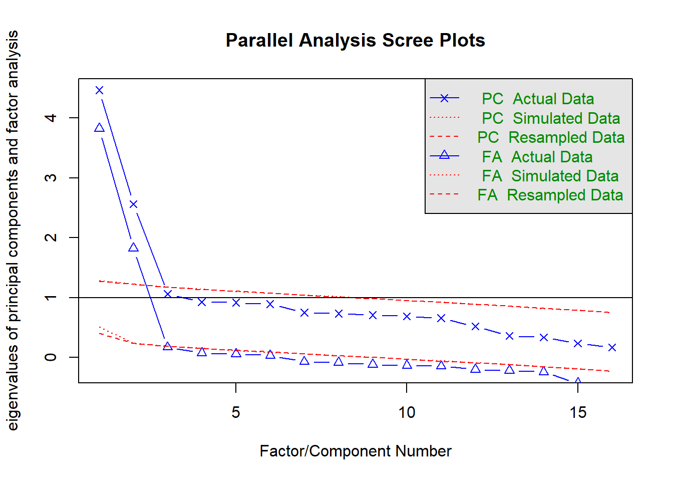
fa.parallel(moodq)

Parallel analysis suggests that the number of factors =  2  and the number of components =  2 

everything points to 2!

We would expect any different dimensions of low mood to be correlated i think:

mood.fa1 <- fa(moodq, nfactors=1)
mood.fa2 <- fa(moodq, nfactors=2, rotate="oblimin",fm="ml")
mood.fa3 <- fa(moodq, nfactors=3, rotate="oblimin",fm="ml")

here i’ve pulled out the variance explained by each solution:

mood.fa1$Vaccounted[2,1]
[1] 0.239
mood.fa2$Vaccounted[3,2]
[1] 0.385
mood.fa3$Vaccounted[3,3]
[1] 0.401

3 factor solution only explains 2% more than the 2 factor solution.
the 3rd factor has no items with it as the primary loading. Pretty clear sign of over-extraction here.

mood.fa3$loadings

Loadings:
       ML1    ML2    ML3   
item1   0.392              
item2   0.956              
item3   0.840              
item4   0.712              
item5   0.356         0.122
item6   0.446         0.182
item7   0.653        -0.254
item8   0.376  0.256       
item9   0.398              
item10         0.908       
item11         0.390  0.246
item12         0.323       
item13         0.785       
item14  0.217  0.378       
item15         0.826       
item16         0.347 -0.218

                 ML1   ML2   ML3
SS loadings    3.385 2.711 0.252
Proportion Var 0.212 0.169 0.016
Cumulative Var 0.212 0.381 0.397

The 1 factor solution explains quite a bit less variance than the 2 factor solution (24% vs 39%).
We have a lot more items with no salient loading in the 1-factor solution, whereas the 2-factor solution every item has a loading \(\geq |.3|\)

print(mood.fa1$loadings, cutoff=.3)

Loadings:
       MR1  
item1  0.334
item2  0.822
item3  0.760
item4  0.639
item5  0.325
item6  0.408
item7  0.569
item8  0.522
item9  0.345
item10 0.497
item11      
item12      
item13 0.505
item14 0.442
item15 0.456
item16      

                 MR1
SS loadings    3.825
Proportion Var 0.239
print(mood.fa2$loadings, cutoff=.3)

Loadings:
       ML1    ML2   
item1   0.398       
item2   0.963       
item3   0.827       
item4   0.706       
item5   0.340       
item6   0.422       
item7   0.680       
item8   0.382       
item9   0.388       
item10         0.902
item11         0.411
item12         0.323
item13         0.784
item14         0.382
item15         0.833
item16         0.324

                 ML1  ML2
SS loadings    3.370 2.71
Proportion Var 0.211 0.17
Cumulative Var 0.211 0.38

mood.fa2
Factor Analysis using method =  ml
Call: fa(r = moodq, nfactors = 2, rotate = "oblimin", fm = "ml")
Standardized loadings (pattern matrix) based upon correlation matrix
         ML1   ML2   h2    u2 com
item1   0.40 -0.05 0.15 0.849 1.0
item2   0.96 -0.02 0.92 0.082 1.0
item3   0.83  0.02 0.69 0.307 1.0
item4   0.71  0.01 0.50 0.499 1.0
item5   0.34  0.02 0.12 0.881 1.0
item6   0.42  0.04 0.19 0.812 1.0
item7   0.68 -0.03 0.45 0.547 1.0
item8   0.38  0.25 0.25 0.746 1.7
item9   0.39 -0.02 0.15 0.853 1.0
item10 -0.02  0.90 0.81 0.194 1.0
item11 -0.03  0.41 0.16 0.836 1.0
item12  0.05  0.32 0.11 0.886 1.0
item13  0.05  0.78 0.63 0.366 1.0
item14  0.21  0.38 0.23 0.772 1.6
item15 -0.04  0.83 0.68 0.320 1.0
item16 -0.01  0.32 0.10 0.896 1.0

                       ML1  ML2
SS loadings           3.41 2.75
Proportion Var        0.21 0.17
Cumulative Var        0.21 0.38
Proportion Explained  0.55 0.45
Cumulative Proportion 0.55 1.00

 With factor correlations of 
     ML1  ML2
ML1 1.00 0.24
ML2 0.24 1.00

Mean item complexity =  1.1
Test of the hypothesis that 2 factors are sufficient.

df null model =  120  with the objective function =  5.47 with Chi Square =  3352
df of  the model are 89  and the objective function was  0.16 

The root mean square of the residuals (RMSR) is  0.03 
The df corrected root mean square of the residuals is  0.03 

The harmonic n.obs is  620 with the empirical chi square  101  with prob <  0.19 
The total n.obs was  620  with Likelihood Chi Square =  101  with prob <  0.19 

Tucker Lewis Index of factoring reliability =  0.995
RMSEA index =  0.014  and the 90 % confidence intervals are  0 0.027
BIC =  -472
Fit based upon off diagonal values = 0.99
Measures of factor score adequacy             
                                                   ML1  ML2
Correlation of (regression) scores with factors   0.97 0.95
Multiple R square of scores with factors          0.94 0.90
Minimum correlation of possible factor scores     0.89 0.80
  • Both factors load on 3+ items at a salient level (\(\geq |.3|\)).
  • There are no Heywood cases.
  • Factors positively correlated 0.24
  • Items 8 and 14 are a bit more complex.
  • The solution explains 38% of the variance.

Here are the wordings of items for factor 1:

names(petdata)[3:11]
[1] "little_interest_or_pleasure_in_doing_things"                                                                                                                          
[2] "feeling_down_depressed_or_hopeless"                                                                                                                                   
[3] "trouble_falling_or_staying_asleep_or_sleeping_too_much"                                                                                                               
[4] "feeling_tired_or_having_little_energy"                                                                                                                                
[5] "poor_appetite_or_overeating"                                                                                                                                          
[6] "feeling_bad_about_yourself_or_that_you_are_a_failure_or_have_let_yourself_or_your_family_down"                                                                        
[7] "trouble_concentrating_on_things_such_as_reading_the_newspaper_or_watching_television"                                                                                 
[8] "moving_or_speaking_so_slowly_that_other_people_could_have_noticed_or_the_opposite_being_so_fidgety_or_restless_that_you_have_been_moving_around_a_lot_more_than_usual"
[9] "a_lack_of_motivation_to_do_anything_at_all"                                                                                                                           

and for factor 2:

names(petdata)[12:18]
[1] "feeling_nervous_anxious_or_on_edge"               
[2] "not_being_able_to_stop_or_control_worrying"       
[3] "worrying_too_much_about_different_things"         
[4] "trouble_relaxing"                                 
[5] "being_so_restless_that_it_is_hard_to_sit_still"   
[6] "becoming_easily_annoyed_or_irritable"             
[7] "feeling_afraid_as_if_something_awful_might_happen"

it kind of makes sense that these two are have higher cross-loadings - they seem to be tapping into something about restlessness:

names(petdata)[c(10,16)]
[1] "moving_or_speaking_so_slowly_that_other_people_could_have_noticed_or_the_opposite_being_so_fidgety_or_restless_that_you_have_been_moving_around_a_lot_more_than_usual"
[2] "being_so_restless_that_it_is_hard_to_sit_still"                                                                                                                       

Replicability

Question 2

Splitting the dataset in two, calculate congruence coefficients for your factor solution.

The most reliable way to split a dataset is actually to create a sample of rows.
For example, if I had 100 rows, then I can split it into two groups of 50 using:

idx <- sample(1:100, 50) # sample 50 rows
split1 <- data[idx, ] # choose those rows
split2 <- data[-idx, ] # exclude those rows

To calculate congruence coefficients, fit the same factor solution to both datasets and then use fa.congruence()

We have 620, so:

idx <- sample(1:620, 310)
df1 <- moodq[idx,]
df2 <- moodq[-idx,]

f1 <- fa(df1, nfactors = 2, rotate = "oblimin", fm = "ml")
f2 <- fa(df2, nfactors = 2, rotate = "oblimin", fm = "ml")
factor.congruence(f1,f2)
     ML1  ML2
ML1 0.99 0.11
ML2 0.00 0.98

Question 3

Ideally, we would split a dataset in two right at the start, develop our model on the “exploratory” half, and not touch the second half of the data until we want to assess congruence.

If we had unlimited time and resources, we would just collect another, completely independent, sample.
So let’s pretend that’s exactly what we’ve done!

You can find a 2nd dataset at https://uoepsy.github.io/data/petmoods_conf.csv that contains the same questions.
Compute congruence coefficients for your factor solution across the two dataset (the first one with n=620 and this one with n=203).

The congruence here is lower, especially for the second factor.
Note that, for instance, item11 is no longer loading onto this factor.

testdat <- read_csv("https://uoepsy.github.io/data/petmoods_conf.csv")
names(testdat)[1:16]<-paste0("item",1:16)

testfa <- fa(testdat[,-17], nfactors = 2, rotate = "oblimin", fm = "ml")

factor.congruence(mood.fa2, testfa)
     ML1  ML2
ML1 0.96 0.11
ML2 0.04 0.85

Reliability

Question 4

Calculate two measures of reliability for each factor - \(alpha\) and \(omega\). How do they differ?

(If you’re thinking “which one should I use?” then there’s not really a right answer - they rely on assuming different measurement models. If you’re going to use mean/sum scores, then reporting reliabilty as \(\alpha\) will make more sense)

Make sure to do this separately for each factor, because both \(\alpha\) and \(\omega_{total}\) assume unidimensionality

alpha(moodq[,1:9])$total
 raw_alpha std.alpha G6(smc) average_r  S/N    ase mean    sd median_r
     0.803      0.81   0.817     0.321 4.25 0.0117 4.09 0.703    0.293
alpha(moodq[,10:16])$total
 raw_alpha std.alpha G6(smc) average_r  S/N    ase mean    sd median_r
     0.761     0.764   0.769     0.316 3.23 0.0144 4.05 0.735    0.294
library(MBESS)
ci.reliability(moodq[,1:9])$est
[1] 0.816
ci.reliability(moodq[,10:16])$est
[1] 0.785

differences in reliability here are quite small!

Getting Scores

Question 5

We’re going to demonstrate how these decisions can have a bearing on your analysis.

Remember, we’re interested in ultimately doing a group comparison (pet owners vs non-pet owners) in the dimension(s) of low mood.

So we’re going to need numbers to give each person’s standing on ‘low mood’ dimension(s).

For each of your factors, create two scores: first calculate a sum score from the relevant items, and then estimate a factor score using factor.scores

  • We’re essentially asking low mood ~ petownership, so the dimensions of low mood are dependent variables. So use the Bartlett method of estimating scores.
  • You’ll probably want to append them to the end of the original dataset where we have the variable about pet ownership.

petdata <- petdata |>
  mutate(
    w.dep=factor.scores(moodq, mood.fa2,method="Bartlett")$scores[,1],
    w.anx=factor.scores(moodq, mood.fa2,method="Bartlett")$scores[,2],
    dep = rowSums(moodq[,1:9]),
    anx = rowSums(moodq[,10:16])
  )

Question 6

Conduct a \(t\)-test to examine whether the pet-owners differ from non-pet-owners in their levels of each factor of low mood.

Try doing this with the sum scores, and then with the factor scores. What is different?

(If you’re wondering “which one is right?” then the answer is kind of “both”/“neither”! Just like \(\alpha\) and \(\omega\), they are assuming different measurement models of the two dimensions)
t.test(dep ~ do_you_own_a_pet, data = petdata)

    Welch Two Sample t-test

data:  dep by do_you_own_a_pet
t = -0.7, df = 610, p-value = 0.5
alternative hypothesis: true difference in means between group 0 and group 1 is not equal to 0
95 percent confidence interval:
 -1.341  0.656
sample estimates:
mean in group 0 mean in group 1 
           36.6            37.0 
t.test(w.dep ~ do_you_own_a_pet, data = petdata)

    Welch Two Sample t-test

data:  w.dep by do_you_own_a_pet
t = -0.5, df = 608, p-value = 0.6
alternative hypothesis: true difference in means between group 0 and group 1 is not equal to 0
95 percent confidence interval:
 -0.203  0.121
sample estimates:
mean in group 0 mean in group 1 
        -0.0204          0.0207 
t.test(anx ~ do_you_own_a_pet, data = petdata)

    Welch Two Sample t-test

data:  anx by do_you_own_a_pet
t = 2, df = 617, p-value = 0.06
alternative hypothesis: true difference in means between group 0 and group 1 is not equal to 0
95 percent confidence interval:
 -0.043  1.575
sample estimates:
mean in group 0 mean in group 1 
           28.8            28.0 
t.test(w.anx ~ do_you_own_a_pet, data = petdata)

    Welch Two Sample t-test

data:  w.anx by do_you_own_a_pet
t = 3, df = 616, p-value = 0.01
alternative hypothesis: true difference in means between group 0 and group 1 is not equal to 0
95 percent confidence interval:
 0.0489 0.3803
sample estimates:
mean in group 0 mean in group 1 
          0.107          -0.108