W4 Exercises: Centering

Hangry

Data: hangry1.csv

The study is interested in evaluating whether levels of hunger are associated with levels of irritability (i.e., “the hangry hypothesis”). 81 participants were recruited into the study. Once a week for 5 consecutive weeks, participants were asked to complete two questionnaires, one assessing their level of hunger, and one assessing their level of irritability. The time and day at which participants were assessed was at a randomly chosen hour between 7am and 7pm each week.

The data are available at: https://uoepsy.github.io/data/hangry1.csv.

variable description
q_irritability Score on irritability questionnaire (0:100)
q_hunger Score on hunger questionnaire (0:100)
ppt Participant
Question 1

Remember that what we’re interested in is “whether levels of hunger are associated with levels of irritability (i.e.,”the hangry hypothesis”)“.

Read in the data and fit the model below. How well does it address the research question?

mod1 <- lmer(q_irritability ~ q_hunger + 
                (1 + q_hunger | ppt), 
                data = hangry)

Always plot your data! It’s tempting to just go straight to interpreting coefficients of this model, but in order to understand what a model says we must have a theory about how the data are generated.

hangry <- read_csv("https://uoepsy.github.io/data/hangry1.csv")

mod1 <- lmer(q_irritability ~ q_hunger + 
                (1 + q_hunger | ppt), 
                data = hangry)

The model above will give us that same old formulaic expression of “for people on average, a 1 unit increase in q_hunger is associated with a 0.17 increase in q_irritability”.

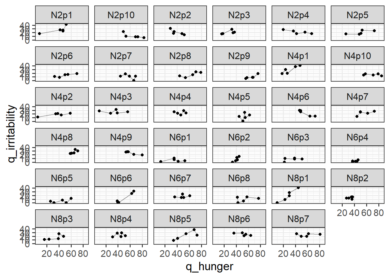
The problem is that in trying to estimate what do as q_hunger increases, we’re ignoring the fact that people tend to have different average levels of q_hunger:

ggplot(hangry, aes(x = q_hunger, y = q_irritability, group = ppt)) +
  geom_point() +
  geom_line(alpha=.4) + 
  facet_wrap(~ppt)

So the interpretation of the fixed effect of our model above as “what happens to a persons’ irritability when they are 1 more hungry?”, we’re not accurately estimating this because our model doesn’t account for the fact that the numbers in q_hunger mean very different things for different people - for person 1 a hunger score of 60 might be “I’m really hungry”, but for person 2 (who is usually in the 80s or 90s) it could mean “I’m not very hungry at all”.

Question 2

Research Question: “whether levels of hunger are associated with levels of irritability (i.e.,”the hangry hypothesis”)“.

Think about the relationship between irritability and hunger. How should we interpret this research aim?

Is it:

  1. “Are people more irritable if they are, on average, more hungry than other people?”
  2. “Are people more irritable if they are, for them, more hungry than they usually are?”
  3. Some combination of both a. and b.

This is just one demonstration of how the statistical methods we use can constitute an integral part of our development of a research project, and part of the reason that data analysis for scientific cannot be so easily outsourced after designing the study and collecting the data.

As our data currently is currently stored, the relationship between irritability and the raw scores on the hunger questionnaire q_hunger represents some ‘total effect’ of hunger on irritability. This is a bit like interpretation c. above - it’s a composite of both the ‘within’ ( b. ) and ‘between’ ( a. ) effects. The problem with this is that this isn’t necessarily all that meaningful. It may tell us that ‘being higher on the hunger questionnaire is associated with being more irritable’, but how can we apply this information? It is not specifically about the comparison between hungry people and less hungry people, and nor is it a good estimation of how person \(i\) changes when they are more hungry than usual. It is both these things smushed together.

To disaggregate the ‘within’ and ‘between’ effects of hunger on irritability, we can group-mean center. For ‘between’, we are interested in how irritability is related to the average hunger levels of a participant, and for ‘within’, we are asking how irritability is related to a participants’ relative levels of hunger (i.e., how far above/below their average hunger level they are.).

Add to the data these two columns:

  1. a column which contains the average hungriness score for each participant.
  2. a column which contains the deviation from each person’s hunger score to that person’s average hunger score.

You’ll find group_by() |> mutate() very useful here, as seen in Chapter 10 #group-mean-centering.

hangry <- 
    hangry |> group_by(ppt) |>
        mutate(
            avg_hunger = mean(q_hunger),
            hunger_gc = q_hunger - avg_hunger
        )
head(hangry)
# A tibble: 6 × 5
# Groups:   ppt [2]
  q_irritability q_hunger ppt   avg_hunger hunger_gc
           <dbl>    <dbl> <chr>      <dbl>     <dbl>
1             42       52 N2p1        39.2     12.8 
2             24       47 N2p1        39.2      7.8 
3             17        8 N2p1        39.2    -31.2 
4             26       47 N2p1        39.2      7.8 
5             27       42 N2p1        39.2      2.80
6             17       48 N2p2        39.6      8.4 

Question 3

For each of the new variables you just added, plot the irritability scores against those variables.

  • Does it look like hungry people are more irritable than less hungry people?
  • Does it look like when people are more hungry than normal, they are more irritable?

You might find stat_summary() useful here for plotting the between effect (see Chapter 10 #group-mean-centering)

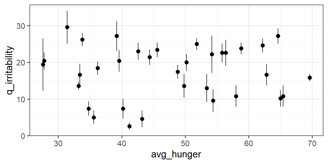
We might find it easier to look at a plot where each participant is represented as their mean plus an indication of their range of irritability scores:

ggplot(hangry,aes(x=avg_hunger,y=q_irritability))+
    stat_summary(geom="pointrange")

It’s hard to see any clear relationship between a persons’ average hunger and their irritability scores here.

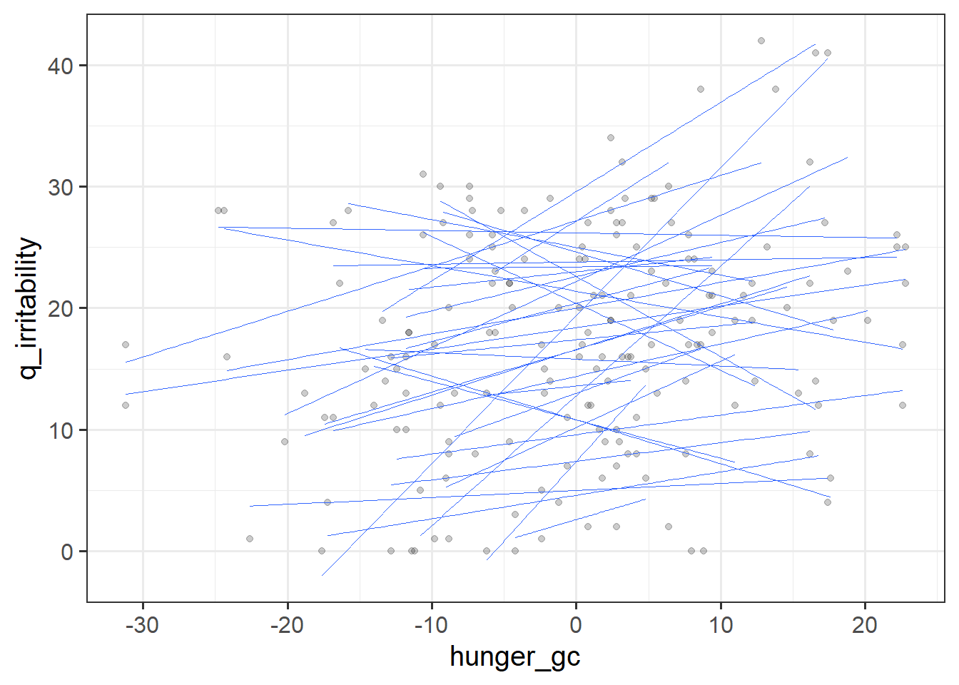
It is also a bit difficult to get at the relationship between participant-centered hunger and irritability, because there are a lot of different lines (one for each participant). To make it easier to get an idea of what’s happening, we’ll make the plot fit a simple lm() (a straight line) for each participants’ data.

ggplot(hangry,aes(x=hunger_gc,y=q_irritability, group=ppt)) +
  geom_point(alpha = .2) + 
  geom_smooth(method=lm, se=FALSE, lwd=.2)

It looks like most of these lines are going upwards, but there’s a fair bit of variation in them.

So we can actually make a guess at what we’re going to see when we model. We’ll probably have a positive fixed effect of hunger_gc (i.e. A below will be positive), and there by-participant variation in these slopes will be quite large relative to the fixed effect (i.e B below will be quite large in comparison to A)

Random effects:
 Groups   Name        Variance Std.Dev. Corr 
 ppt      (Intercept)      ...      ... 
          hunger_gc        ...      *B*
 Residual                  ...      ...    

...

Fixed effects:
            Estimate Std. Error t value
(Intercept)      ...        ...     ...
hunger_gc        *A*        ...     ...
...              ...        ...     ...

Question 4

We have taken the raw hunger scores and separated them into two parts (raw hunger scores = participants’ average hunger score + observation level deviations from those averages), that represent two different aspects of the relationship between hunger and irritability.

Adjust your model specification to include these two separate variables as predictors, instead of the raw hunger scores.

  • We can only put one of these variables in the random effects (1 + hunger | participant). Think about the fact that each participant has only one value for their average hungriness.
  • If the model fails to converge, and it’s a fairly simple model (i.e one or two random slopes), then often you can switch optimizer (see Chapter 2 #convergence-warnings-singular-fits). For instance, try adding control = lmerControl(optimizer = "bobyqa") to the model.

With the defaults, this model doesn’t converge

hangrywb <- lmer(q_irritability ~ avg_hunger + hunger_gc + 
                (1 + hunger_gc | ppt), 
                data = hangry)

Changing the optimizer helps:

hangrywb <- lmer(q_irritability ~ avg_hunger + hunger_gc + 
                (1 + hunger_gc | ppt), 
                data = hangry,
                control = lmerControl(optimizer = "bobyqa"))

Note that the max|grad| convergence error of the initial model was very close to the tolerance (see Chapter 8 #non-convergence for an explanation of what this tolerance is).

The fact that it is close indicates that we may be quite close to a solution, so it’s worth investigating if this is simply an optimizer problem.

One other thing to do would be to consider all available optimizers, see which ones converge, and compare estimates across them. If the estimates are the same (or pretty close), and some of these converge, then it gives us more trust in our model. We can do this with the code below. We can see that 5 optimizers don’t give error messages, and that they all give pretty much the same estimated fixed effects. We can go further and compare random effects variances too, but we won’t do that here.

# fit with all optimizers
allopts = allFit(hangrywb)
bobyqa : [OK]
Nelder_Mead : [OK]
nlminbwrap : [OK]
nloptwrap.NLOPT_LN_NELDERMEAD : [OK]
nloptwrap.NLOPT_LN_BOBYQA : 
[OK]
# error messages from each optimizer 
# (NULL here means no message, which is good)
summary(allopts)$msgs
$bobyqa
NULL

$Nelder_Mead
NULL

$nlminbwrap
NULL

$nloptwrap.NLOPT_LN_NELDERMEAD
NULL

$nloptwrap.NLOPT_LN_BOBYQA
[1] "Model failed to converge with max|grad| = 0.0027028 (tol = 0.002, component 1)"
# fixed effect estimates for all optimizers
summary(allopts)$fixef
                              (Intercept) avg_hunger hunger_gc
bobyqa                               17.6   -0.00644     0.187
Nelder_Mead                          17.6   -0.00644     0.187
nlminbwrap                           17.6   -0.00644     0.187
nloptwrap.NLOPT_LN_NELDERMEAD        17.6   -0.00647     0.187
nloptwrap.NLOPT_LN_BOBYQA            17.6   -0.00648     0.187

Question 5

Write down an interpretation of each of the fixed effects

Here they are

fixef(hangrywb)
(Intercept)  avg_hunger   hunger_gc 
   17.62005    -0.00644     0.18663 
term est interpretation
(Intercept) 17.620 estimated irritability score for someone with an average hunger of 0, and not deviating from that average (i.e. hunger_gc = 0)
avg_hunger -0.006 estimated difference in irritability between two people who differ in average hunger level by 1 (e.g., a person with average hunger of 11 vs someone with average hunger level of 10), when they are at their average (hunger_gc = 0)
hunger_gc 0.187 estimated change in irritability score for every 1 more hungry a person is than they normally are

Question 6

Have a go at also writing an explanation for yourself of the random effects part of the output.
There’s no formulaic way to interpret these, but have a go at describing in words what they represent, and how that adds to the picture your model describes.

Don’t worry about making it read like a report - just write yourself an explanation!

VarCorr(hangrywb)
 Groups   Name        Std.Dev. Corr 
 ppt      (Intercept) 6.992         
          hunger_gc   0.366    -0.08
 Residual             4.772         
term est interpretation
sd__(Intercept) 6.992 Participant level variability in irritability when they are at their average hunger level - i.e. when everybody is at their own average level of hunger, they vary in their irritability scores with a standard deviation of 7.
sd__hunger_gc 0.366 Participants vary quite a bit in how deviations from hunger are associated with irritability. They vary around the fixed effect of 0.19 with a standard deviation of 0.37. To think about what this means, imagine a normal distribution that is centered on 0.19 and has a standard deviation of 0.36. A fairly large portion of that distribution would fall below zero (i.e. have a negative slope). And we would also expect some slopes that are e.g., .5, .6 etc
cor__(Intercept).hunger_gc -0.080 this estimate is basically zero, but represents the relationship between participants relative standing at the intercept and their relative standing on the slopes. So participants who are more irritable than others when at their average hunger, tend to have slightly lower slopes
sd__Observation 4.772 the residual variance doesn't really have much of an interpretation - it really just represents all the leftover stuff that the model doesn't explain. If we imagine all of the individual participant lines, this represents how spread out the individual observations are around those lines

Hangry 2

Question 7

A second dataset on the same variables is available at: https://uoepsy.github.io/data/hangry2.csv.
These data are from people who were following a five-two diet, while the original dataset were from people who were not folling any diet.

Combine the datasets together so we can fit a model to see if the hangry effect differs between people on diets vs those who aren’t.

  • Something like bind_rows() might help here. If you’ve not seen it before, remember that you can look up the help documentation in the bottom-right panel of RStudio
  • Be sure to keep an indicator of which group the data are in!!

Here are our two datasets:

hangry1 <- read_csv("https://uoepsy.github.io/data/hangry1.csv")
hangry2 <- read_csv("https://uoepsy.github.io/data/hangry2.csv")

We could simply bind them together using bind_rows()

hangryfull <- 
  bind_rows(
    hangry1, 
    hangry2
  )

but then we wouldn’t know who was from which group! So we’ll need to add a variable to each one first:

hangryfull <- 
  bind_rows(
    hangry1 |> mutate(diet = "N"), 
    hangry2 |> mutate(diet = "Y")
  )
head(hangryfull)
# A tibble: 6 × 4
  q_irritability q_hunger ppt   diet 
           <dbl>    <dbl> <chr> <chr>
1             42       52 N2p1  N    
2             24       47 N2p1  N    
3             17        8 N2p1  N    
4             26       47 N2p1  N    
5             27       42 N2p1  N    
6             17       48 N2p2  N    

Question 8

Does the relationship between hunger and irritability depend on whether or not people are following the five-two diet?

Which relationship between hunger and irritability are we talking about? The between effect or the within effect? It could be both!
We’re going to need to create those two variables again for this combined dataset.

hangryfull <- 
    hangryfull |> group_by(ppt) |>
        mutate(
            avg_hunger = mean(q_hunger),
            hunger_gc = q_hunger - avg_hunger
        )

hangrywbdiet <- lmer(q_irritability ~ (avg_hunger + hunger_gc) * diet + 
                (1 + hunger_gc | ppt), 
                data = hangryfull,
                control=lmerControl(optimizer="bobyqa"))

summary(hangrywbdiet)
Linear mixed model fit by REML ['lmerMod']
Formula: q_irritability ~ (avg_hunger + hunger_gc) * diet + (1 + hunger_gc |  
    ppt)
   Data: hangryfull
Control: lmerControl(optimizer = "bobyqa")

REML criterion at convergence: 2735

Scaled residuals: 
    Min      1Q  Median      3Q     Max 
-2.4138 -0.5906 -0.0454  0.5426  2.3954 

Random effects:
 Groups   Name        Variance Std.Dev. Corr 
 ppt      (Intercept) 48.083   6.934         
          hunger_gc    0.145   0.381    -0.01
 Residual             23.305   4.828         
Number of obs: 405, groups:  ppt, 81

Fixed effects:
                  Estimate Std. Error t value
(Intercept)       17.13095    5.14648    3.33
avg_hunger         0.00386    0.10533    0.04
hunger_gc          0.18577    0.07560    2.46
dietY            -10.85470    6.53568   -1.66
avg_hunger:dietY   0.46590    0.13354    3.49
hunger_gc:dietY    0.38141    0.10139    3.76

Correlation of Fixed Effects:
            (Intr) avg_hn hngr_g dietY  avg_:Y
avg_hunger  -0.971                            
hunger_gc   -0.002  0.000                     
dietY       -0.787  0.765  0.002              
avg_hngr:dY  0.766 -0.789  0.000 -0.968       
hngr_gc:dtY  0.002  0.000 -0.746 -0.002  0.000

Question 9

Construct two plots showing the two model estimated interactions. This model is a bit of a confusing one, so plotting may help a bit with understanding what those interactions represent.

  • effects(terms, mod) |> as.data.frame() |> ggplot(.....)

The xlevels bit here just gives us the little dataframe to plot with more levels at it, so that it gives us smoother lines. Try it with and without to see what I mean!

library(effects)
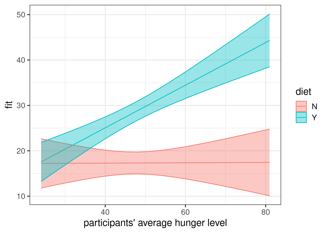
effect("avg_hunger*diet", hangrywbdiet, xlevels=20) |>
  as.data.frame() |>
  ggplot(aes(x=avg_hunger, y=fit,col=diet))+
  geom_line()+
  geom_ribbon(aes(ymin=lower,ymax=upper,fill=diet),alpha=.4)+
  labs(x="participants' average hunger level")

We saw in our original model that for the reference level of diet, the “N” group, there was no association between how hungry a person is on average and their irritability. This is the red line we see in the plot above. In our full model this is the avg_hunger coefficient.

We also saw the interaction avg_hunger:dietY indicates that irritability is estimated to increase by 0.47 more for those in the diet than it does for those not on the diet. So the blue line is should be going up more steeply than the red line (which is flat). And it is!

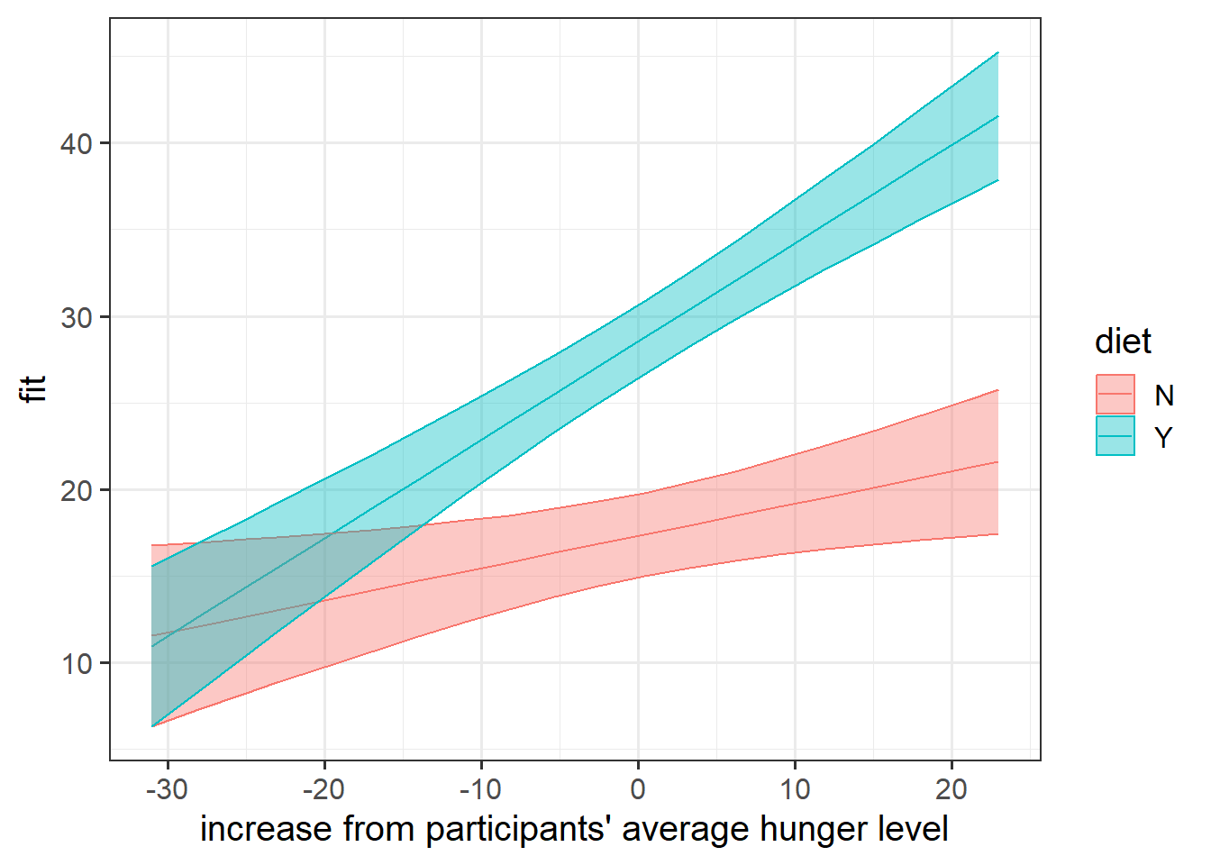
effect("hunger_gc*diet", hangrywbdiet, xlevels=20) |>
  as.data.frame() |>
  ggplot(aes(x=hunger_gc, y=fit,col=diet))+
  geom_line()+
  geom_ribbon(aes(ymin=lower,ymax=upper,fill=diet),alpha=.4)+
  labs(x="increase from participants' average hunger level")

From the coefficient of hunger_gc we get the estimated amount by which irritability increases for every 1 more hungry that a person becomes (when they’re in the diet “N” group). This is the slope of the red line - the hunger_gc coefficient from our full model.
The interaction hunger_gc:fivetwo1 gave us the adjustment to get from the red line to the blue line. It is positive which matches with the fact that the blue line is steeper in this plot.

Question 10

Provide tests of the fixed effects and write-up the results.
hangrywbdiet.p <- lmerTest::lmer(q_irritability ~ (avg_hunger + hunger_gc) * diet + 
                (1 + hunger_gc | ppt), 
                data = hangryfull,
                control=lmerControl(optimizer="bobyqa"))

summary(hangrywbdiet.p)$coefficients
                  Estimate Std. Error   df t value Pr(>|t|)
(Intercept)       17.13095     5.1465 77.0  3.3287 0.001341
avg_hunger         0.00386     0.1053 77.0  0.0367 0.970834
hunger_gc          0.18577     0.0756 65.4  2.4573 0.016659
dietY            -10.85470     6.5357 77.0 -1.6608 0.100813
avg_hunger:dietY   0.46590     0.1335 77.0  3.4888 0.000806
hunger_gc:dietY    0.38141     0.1014 68.5  3.7617 0.000352

To investigate the association between irritability and hunger, and whether this relationship is different depending on whether or not participants are on a restricted diet such as the five-two, a multilevel linear model was fitted.
To disaggregate between the differences in irritability due to people being in general more/less hungry, and those due to people being more/less hungry than usual for them, irritability was regressed onto both participants’ average hunger scores their relative hunger levels. Both of these were allowed to interact with whether or not participants were on the five-two diet. Random intercepts and slopes of relative-hunger level were included for participants. The model was fitting with restricted maximum likelihood estimation with the lme4 package (Bates et al., 2015), using the bobyqa optimiser from the lme4. \(P\)-values were obtained using the Satterthwaite approximation for degrees of freedom.

Results indicate that for people on no diet, being more hungry than normal was associated with greater irritability (\(b = 0.19,\ SE = 0.08,\ t(65.41) = 2.46,\ p=0.017\)), and that this was increased for those following the five-two diet (\(b = 0.38,\ SE = 0.1,\ t(68.49) = 3.76,\ p<0.001\)). Although for those not on a specific diet there was no evidence for an association between irritability and being generally a more hungry person (\(p=0.971\)), there a significant interaction was found between average hunger and being on the five-two diet (\(b = 0.47,\ SE = 0.13,\ t(77) = 3.49,\ p<0.001\)), suggesting that when dieting, hungrier people tend to be more irritable than less hungry people.
Results suggest that the ‘hangry hypothesis’ may occur within people (when a person is more hungry than they usually are, they tend to be more irritable), but not necessarily between hungry/less hungry people. Dieting was found to increase the association of both between-person hunger and within-person hunger with irritability.