| variable | description |
|---|---|
| age | Age in years of respondent |
| outdoor_time | Self report estimated number of hours per week spent outdoors |
| social_int | Self report estimated number of social interactions per week (both online and in-person) |
| routine | Binary 1=Yes/0=No response to the question 'Do you follow a daily routine throughout the week?' |
| wellbeing | Warwick-Edinburgh Mental Wellbeing Scale (WEMWBS), a self-report measure of mental health and wellbeing. The scale is scored by summing responses to each item, with items answered on a 1 to 5 Likert scale. The minimum scale score is 14 and the maximum is 70 |
| location | Location of primary residence (City, Suburb, Rural) |
| steps_k | Average weekly number of steps in thousands (as given by activity tracker if available) |
08: Assumptions and diagnostics
This week, you’ll revisit a multiple regression model you developed in Block 1. Using that model, you’ll practice checking assumptions and running diagnostics of multicollinearity and influence.
NoteGet set up
- Open RStudio.
- Create a new .Rmd file for this week’s exercises.
- Save it somewhere you can find it again.
- Give it a clear name (for example,
dapr2_lab08.Rmd). - In the first code chunk, load the packages you’ll need this week (and install them if you don’t have them already):
tidyversecar
Research question (RQ): Is there an association between wellbeing and time spent outdoors, when controlling for the effect that social interaction has on wellbeing?
Data dictionary:
NoteMore detail about this dataset
From the Edinburgh & Lothians, 100 city/suburb residences and 100 rural residences were chosen at random and contacted to participate in the study. The Warwick-Edinburgh Mental Wellbeing Scale (WEMWBS) was used to measure mental health and wellbeing.
Participants filled out a questionnaire including items concerning: estimated average number of hours spent outdoors each week, estimated average number of social interactions each week (whether on-line or in-person), whether a daily routine is followed (yes/no). For those respondents who had an activity tracker app or smart watch, they were asked to provide their average weekly number of steps.
Set up data and model
Question 1
We recommend that you copy and paste code that you wrote back in Lab 03 for this question.
Read in the data from https://uoepsy.github.io/data/wellbeing_rural.csv and store it in a variable named mwdata (“mw” stands for “mental wellbeing”).
Fit the linear model represented by the mathematical model formulation below and (unlike Lab 03!) name the result m1.
\[ \text{wellbeing} = \beta_0 + (\beta_1 \cdot \text{outdoor\_time}) + (\beta_2 \cdot \text{social\_int}) + \epsilon \]
Check assumptions
Question 2
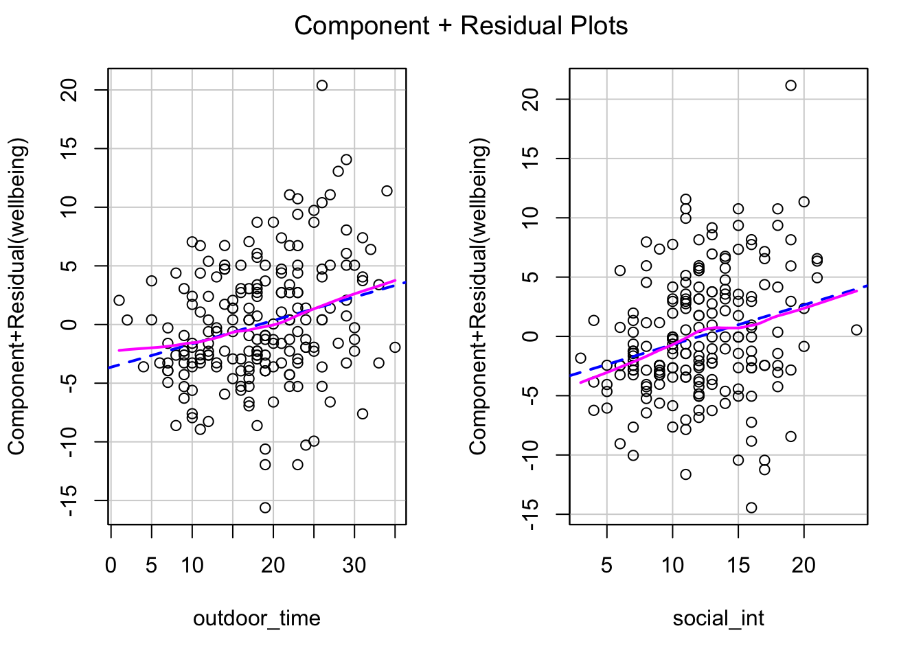
Check: Are you willing to assume that the associations between each predictor and the outcome in m1 are sufficiently linear?
🗂️ See LM assumptions > Linearity of association flash card.
Question 3
Check: Are you willing to assume that the errors in m1 are independent?
🗂️ See LM assumptions > Independence of errors flash card.
Question 4
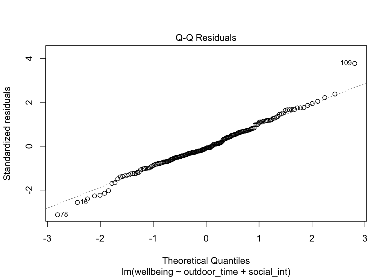
Check: Are you willing to assume that the errors in m1 are sufficiently normally distributed?
🗂️ See LM assumptions > Normality of errors flash card.
Question 5
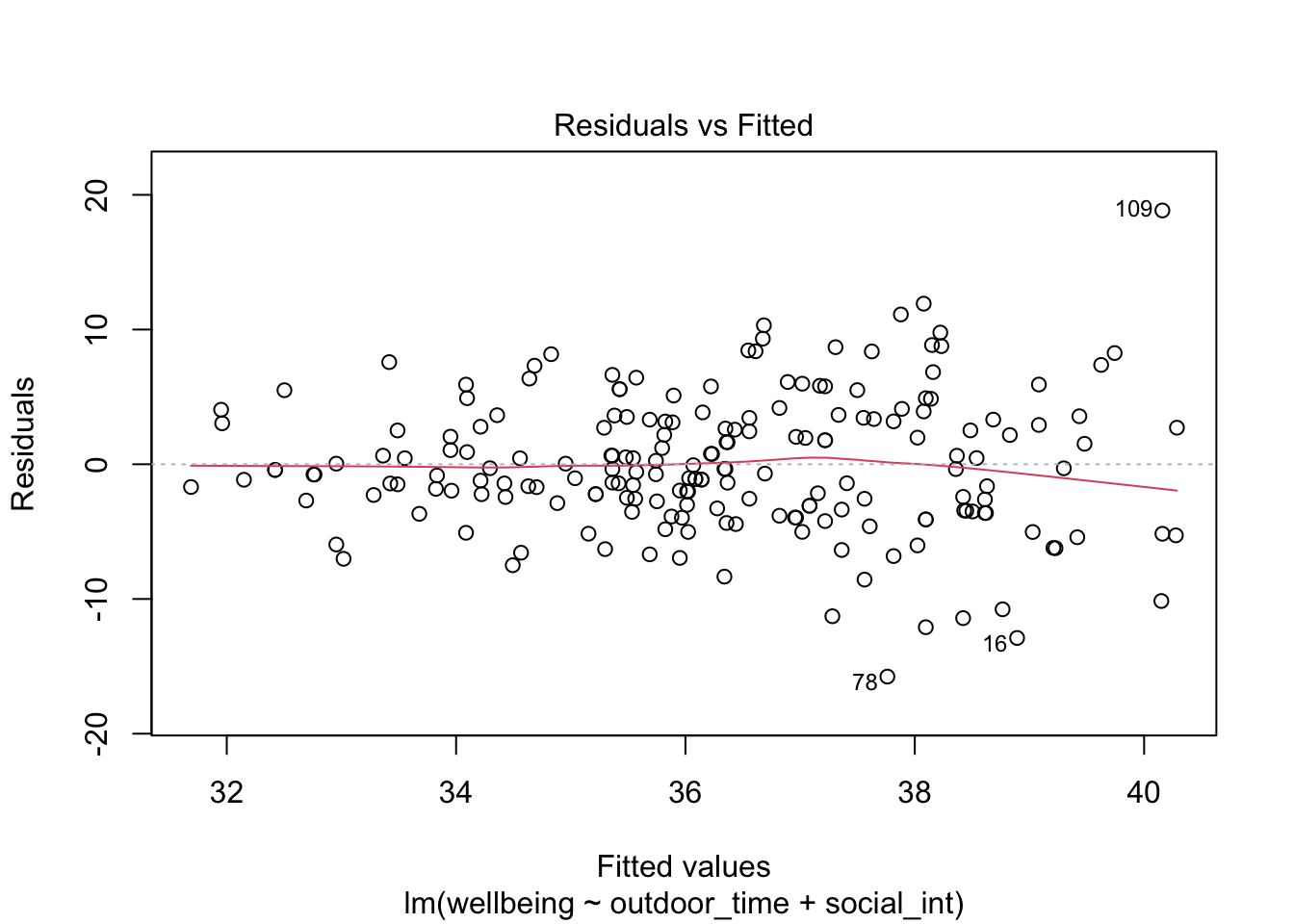
Check: Are you willing to assume that the errors in m1 have sufficiently equal variance across the whole range of fitted values?
🗂️ See LM assumptions > Equal variance of errors flash card.
Check multicollinearity
Question 6
Check: Will multicollinearity between predictors be a problem for m1?
🗂️ See Checking multicollinearity flash card.
Check influence
Question 7
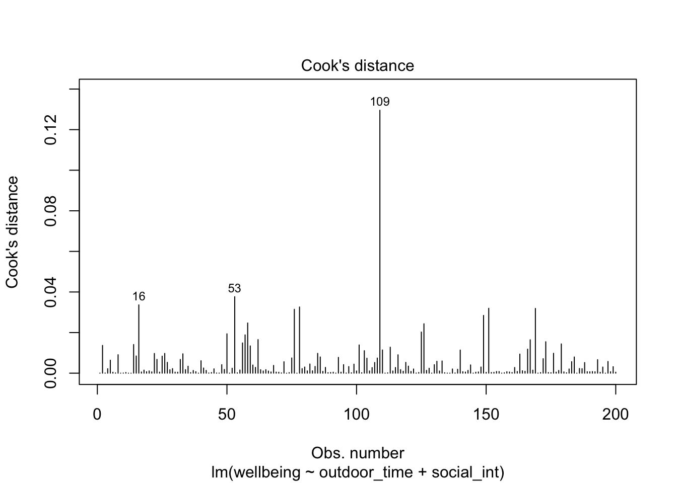
One particular observations influences the model’s estimates more than others.
Check: What row is that observation in?
🗂️ See Influential observations flash card.
Run sensitivity analysis
Question 8
Fit the same model from Q1 to a version of the dataset that does not include the high-influence data point.
Name that model m2.
🗂️ See Sensitivity analysis flash card.
Question 9
This is a conceptual/interpretation question—no coding needed.
Compare the model summaries for m1 and m2.
- Write a sentence to answer: How much do the coefficient estimates change after the high-influence data point has been removed?
- Write a sentence to answer: How much does the pattern of statistical significance change?
🗂️ See Sensitivity analysis flash card.
Question 10
This is a conceptual/interpretation question—no coding needed.
Decide: Does the high-influence observation impact the conclusions you would draw from the model?
🗂️ See Sensitivity analysis flash card.
Optional: Knit your report to PDF
Note: During the labs, please spend your time on the exercises above, not on rendering your document. This guidance is here in case you have extra time at the end.
Rmarkdown is a useful format because it can be used as a foundation for generating different kinds of documents. For the group report, you’ll be asked to render your Rmd file to PDF. Why not practice now?
First, make sure you have tinytex installed in R. This is what lets you convert things into PDF format.
Run the following code to install tinytex (you’ll only need to run it once).
install.packages("tinytex")
tinytex::install_tinytex()
Then ensure that the “yaml” (rhymes with “mammal”) header—the bit at the top of your Rmd document—looks something like this:
---
title: "this is my report title"
author: "B1234506"
date: "07/09/2025"
output: bookdown::pdf_document2
---
Then follow the instructions from the Rmd bootcamp to knit your Rmd document to PDF.
If you encounter errors, refer to the DAPR1 formatting resources / knitting checklist.
TipWhat to do if you cannot knit to PDF
If you are having issues knitting directly to PDF, try the following:
- Knit to HTML file
- Open your HTML in a web-browser (e.g. Chrome, Firefox)
- Print to PDF (Ctrl+P, then choose to save to PDF)
- Open file to check formatting
TipHiding code and/or output from code chunks
Review Lesson 5 of the rmd bootcamp for a detailed description/worked examples.
Hiding R Code
To not show the code of an R code chunk, and only show the output, write:
```{r, echo=FALSE}
# code goes here
```
Hiding R Output:
To show the code of an R code chunk, but hide the output, write:
```{r, results='hide'}
# code goes here
```
Hiding R code AND output
To hide both code and output of an R code chunk, write:
```{r, include=FALSE}
# code goes here
```