| Variable | Description |
|---|---|
| FOMO | FOMO Score (as measured by the 10-item FOMO scale) |
| Age | Age (in years) |
| N | Score on personality items assessing Neuroticism from the Big Five Inventory (BFI) |
| E | Score on personality items assessing Extraversion from the Big Five Inventory (BFI) |
| O | Score on personality items assessing Openness from the Big Five Inventory (BFI) |
| A | Score on personality items assessing Agreeableness from the Big Five Inventory (BFI) |
| C | Score on personality items assessing Conscientiousness from the Big Five Inventory (BFI) |
| TotalFollowers | Total Number of Instagram Followers |
05: Practice write-up
This week (and every fifth week this year), you’ll practice writing up the analysis that was developed live during lectures.
Your goal is to present your analysis in a journal-article-style Results section that a reader could reproduce in any statistical software, not just R.
Quick links to key flash cards:
Important
The example write-ups that will be provided on Friday are not perfect.
You must not copy them directly for this write-up or any future assessment, as copying and presenting them as your own work would constitute academic misconduct. But you may refer to them for stylistic guidance.
NoteGet set up
- Open RStudio.
- Create a new R Markdown (.Rmd) file for this week’s exercises.
- Save it somewhere you can find it again.
- Give it a clear name (for example,
dapr2_lab05.Rmd). - In the first code chunk, load the packages you’ll need this week (and install them if you don’t have them already):
tidyversepsychsjPlotkableExtrapatchwork
The data in FOMOdataset.csv contain eight attributes collected from a sample of \(n=3370\) hypothetical individuals across the UK, and include:
NoteMore detail about this dataset
The data used for this write-up exercise are simulated, drawing on recent work on Fear of Missing Out (FOMO), socio-demographic factors, and the Big Five personality traits. The simulated data are based on the findings of this work, and acted to expand upon the methods and results reported in the following paper:
Rozgonjuk, D., Sindermann, C., Elhai, J. D., & Montag, C. (2021). Individual differences in Fear of Missing Out (FOMO): Age, gender, and the Big Five personality trait domains, facets, and items. Personality and Individual Differences, 171, 110546. https://doi.org/10.1016/j.paid.2020.110546
In the current study, participants were invited to an online study investigating the associations among FOMO, socio-demographic factors, and personality. The final sample comprised 3370 people. Participants completed a FOMO scale and a personality inventory. The 10-item FOMO scale measured the extent of experiencing apprehension regarding missing out on interesting events of others on a 5-point scale (1 = “not at all true of me” to 5 = “extremely true of me”), producing a possible range of scores between 10 and 50. The Big Five Inventory (BFI) is a 45-item personality assessment questionnaire (note that only 44 items were used to match the study above) that uses a five-point response scale (1 = “very inapplicable” to 5 = “very applicable”). The BFI consists of five domains: Neuroticism (8 items; possible range of scores 8-40), Extraversion (8 items; possible range of scores 8-40), Openness to Experience (10 items; possible range of scores 10-50), Agreeableness (9 items; possible range of scores 9-45), and Conscientiousness (9 items; possible range of scores 9-45). We extended the aforementioned study to include an extra socio-demographic variable - a measure of popularity on social media based on the number of followers. Unlike the original study, we do not have measures of gender, education level, or specific country of residence.
RQ1
RQ: How is people’s sense of Fear of Missing Out (FOMO) associated with their age and how many Instagram followers they have?
Specific predictions:
- As age increases, FOMO will decrease.
- As the number of Instagram followers increases, FOMO will increase.
TipProvided analysis code for RQ1
This code should resemble the analysis developed during lectures this week.
# RQ1 example code ----

# Follows workflow here: dapr2/2627/dapr2_flashcards/resources/workflow.html

## Phase 1: Before model fitting ----

### 1a: Set up code and data ----

# Load required R packages
library(tidyverse)   # for wrangling
library(psych)       # for summarising
library(sjPlot)      # for nice tables/plots
library(kableExtra)  # for nicely-formatted tables
library(patchwork)   # for combining plots into one graphic


# Read in data
fomo <- read_csv("https://uoepsy.github.io/data/FOMOdataset.csv")


# Tidy data if needed
glimpse(fomo)  # all numeric, so we'll use psych::describe() to look for weird data
describe(fomo)  # min and max look reasonable
table(is.na(fomo))  # no NAs
# good to continue!

### 1b: Set up the variables we'll model ----

# RQ: How is people's sense of Fear of Missing Out (FOMO) associated with their age and how many Instagram followers they have?

# Based on RQ, identify outcome variables and predictors.
# - Outcome: `FOMO`
# - Predictors: `Age`, `TotalFollowers`

# Based on RQ, decide whether to test hypotheses using coefficient significance tests or model comparison.
# - The RQ is about associations between variables, so we'll test it using significance test for coef estimates.

# Set up continuous predictors. (e.g., any transformations?)
# - One option might be to z-score Age and TotalFollowers.
#   This would be an important step if Age = 0 and TotalFollowers = 0 were totally meaningless quantities (imagine Height = 0 or ShoeSize = 0 – impossible and nonexistent).
#   But Age = 0 means an infant, and TotalFollowers = 0 means someone with no followers.
#   So they are reasonable quantities to generate predictions for.

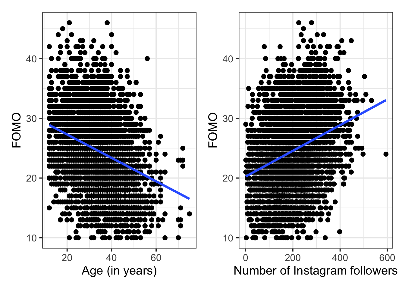
# Explore patterns in the data by plotting outcome and predictor variables together.

p_age <- fomo |>
  ggplot(aes(x = Age, y = FOMO)) +
  geom_point() +
  geom_smooth(method = 'lm', se = FALSE)
p_age

p_followers <- fomo |>
  ggplot(aes(x = TotalFollowers, y = FOMO)) +
  geom_point() +
  geom_smooth(method = 'lm', se = FALSE)
p_followers

p_age + p_followers  # combine using patchwork


## Phase 2: Model fitting ----

# Write the mathematical model formulation for your model(s).
#  $$
#    \text{FOMO} = \beta_0 + (\beta_1 \cdot \text{Age}) + (\beta_2 \cdot \text{Followers}) + \epsilon
#  $$


# Explicitly define the hypotheses that your RQ is aiming to test.
#  $$
#  \begin{align}
#  H_0 &: \text{ All } \beta_j = 0 \text{ for } j = 1, 2 \\
#  H_1 &: \text{ Any } \beta_j \neq 0 \\
#  \end{align}
#  $$

# Fit your model(s) using lm().
m1 <- lm(
  FOMO ~ Age + TotalFollowers,
  data = fomo
)


## Phase 3: After model fitting ----

### 3a: Plot and interpret model estimates ----

# Interpret the coefficient estimates (if appropriate for your RQ).
summary(m1)
confint(m1) |> round(2)
confint(m1) |> round(3)  # for TotalFollowers

# - `Intercept`: The estimated FOMO score for someone aged zero with zero total followers is 26.52 points.
# - `Age`: Increasing one year of age is associated with a decrease in FOMO score of 0.17 points (holding follower count constant). This estimate is significantly different from zero (b = –0.17, 95% CI [–0.18, –0.15], p < .001).
# - prediction supported!
#   - `TotalFollowers`: Increasing one follower is associated with an increase in FOMO score of 0.018 points (holding age constant). This estimate is significantly different from zero (b = 0.018, 95% CI [0.016, 0.020], p < .001).
# - prediction supported!
#   - (rounded to 3 dp because otherwise estim and CI bounds are all 0.02)


# Generate a nicely-formatted regression table (if appropriate for your RQ).
tab_model(
  m1,
  dv.labels = 'Fear of missing out (FOMO)',
  pred.labels = c("Age" = "Age (in years)"),
  title = "RQ1: Linear model coefficient estimates"
)

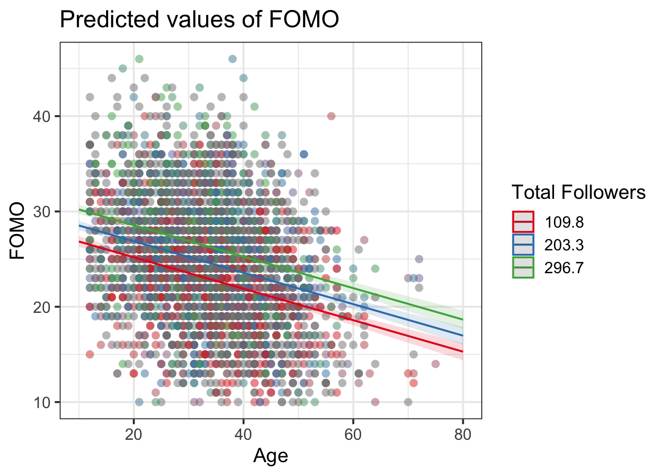
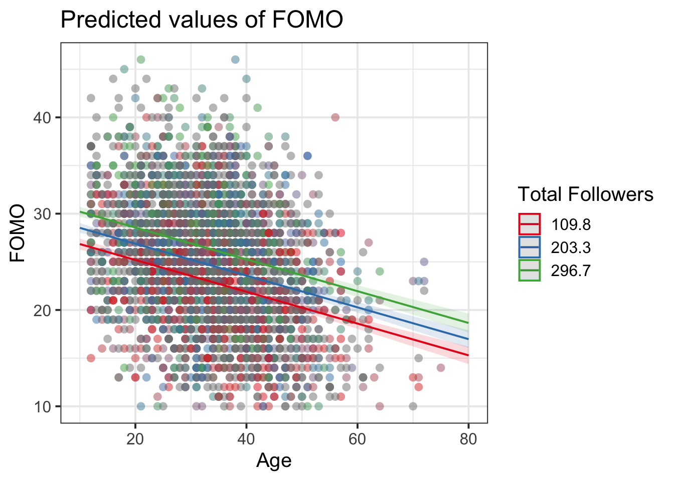
# Plot model-fitted values (if appropriate for your RQ).
plot_model(
  m1,
  type = 'eff',
  terms = c('Age', 'TotalFollowers'),
  show.data = TRUE
)
Question 1
Set the scene (so the reader knows what you’re talking about).
Question 2
Describe and show the sample data (so that the reader knows how generalisable your analysis might be).
Question 3
Visualise and summarise data patterns that address the RQ (so the reader knows the basic pattern of what you found).
-
- Tip: If you transform any continuous predictors for analysis, use the transformed version of the predictor in the plot.
- Tip: In the caption, briefly explain what every geom in the plot represents. Especially error bars/shaded error ribbons! Always tell the reader what they show (standard deviation? standard error? 95% CI?).
- Tip: Academic writing styles vary, but Elizabeth likes it when figure captions give the reader a brief take-home message about what they should see in the plot.
-
- Tip: No inferential stats have been done yet, so we can’t make any claims just yet about whether the predictions were supported. But it is OK to say whether the results appear broadly in line with the prediction.
Question 4
Introduce your statistical analysis (so the reader can interpret the numbers you will report).
Question 5
Report the results of your analysis (so the reader knows exactly what you found).
-
- Tip: You don’t need to report every single parameter estimate. Focus on the one(s) you identified as being relevant to your prediction(s).
- Tip: Briefly link the direction and significance of the effect back to your earlier predictions—is the prediction supported by the parameter estimate?
Common problems in LM write-ups
Below are some examples of common problems we encounter in write-ups of LM analyses. If you want to produce a really clear and strong write-up, then try to avoid these issues. Do any of them appear in the draft you’ve written? If they do, can you edit your draft to solve each one?
Our example solutions, which illustrate how you might get around these problems, will be shared on Friday.
ImportantIncluding too little necessary information
For example:
The first slope was significant (\(b\) = –0.17, 95% CI [–0.18, –0.15], \(p\) < .001). The second slope was also significant (\(b\) = 0.018, 95% CI [0.016, 0.020], \(p\) < .001).
- The reader doesn’t know which one is the slope over age and which is the slope over the number of Instagram followers.
- The reader also doesn’t know what these numbers mean in the context of the analysis. To remedy this, each coefficient must be interpreted in the context of the data (e.g., something like “holding [other variable] constant, increasing one unit of [this variable] is associated with an increase/decrease in [outcome] of [x] points”).
For example:
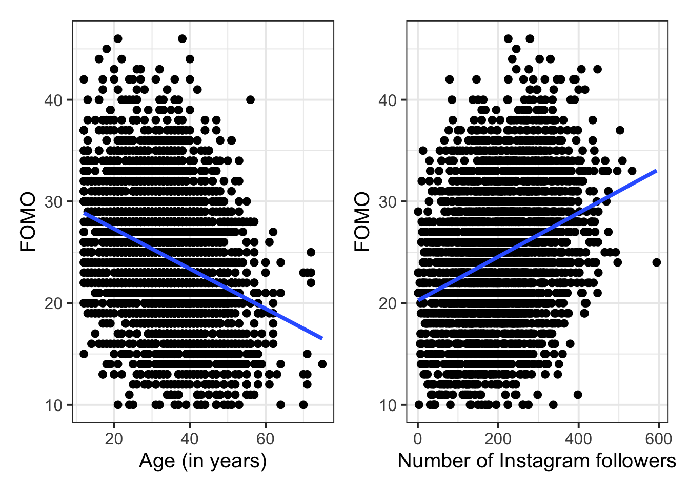
Figure 1: Plot of the data
- What are the variables being plotted?
- What patterns/associations should the reader notice in the plot?
- General figure caption advice: If you were describing this plot in words to somebody who cannot see it, what would you say?
ImportantIncluding too much unnecessary detail
For example:
There are 3370 rows in the dataframe, and each row represents one participant. There was no data cleaning / outlier removal / transformations.”
- The first sentence is all right, but it could be easily shortened to “We have data from 3370 participants”, which is what we actually care about more than the number of rows in the dataframe.
- If a particular analysis step is not applicable, then you don’t need to mention that you didn’t do it.
For example:
The predictions were supported. \(\beta_0\) shows that the estimated mean FOMO score for people aged zero with no followers is 26.52 points. \(\beta_1\) shows […]
- The intercept \(\beta_0\) was not involved in any of our predictions, so you don’t need to spend your valuable word count on reporting it in a sentence. It’ll appear anyway in the regression coefficient table, so the readers will still see what it is, and they can interpret it themselves if they want to.
ImportantUsing R variable names and R notation in the text
For example:
The dataset contains the variables FOMO, Age, TotalFollowers, N, E, O, A, and C.
- Describe in natural English / human-readable language what the variables mean, not what they’re called in our specific dataset.
- Your goal is to describe the dataset so that somebody who doesn’t have access to it could, in principle, collect data on the exact same variables.
For example:
The model is FOMO ~ Age + TotalFollowers.
- Write out the model structure in words and mathematical notation, not R syntax.
- Your goal is to be able to convey the model’s structure even to readers who are using statistical software that is not R.
ImportantUninformative or inaccessible colour in plots
For example:
Code
p_age <- fomo |>
    ggplot(aes(x = Age, y = FOMO)) +
    geom_point(colour="limegreen")
p_followers <- fomo |>
    ggplot(aes(x = TotalFollowers, y = FOMO)) +
    geom_point(colour="limegreen")

p_age + p_followers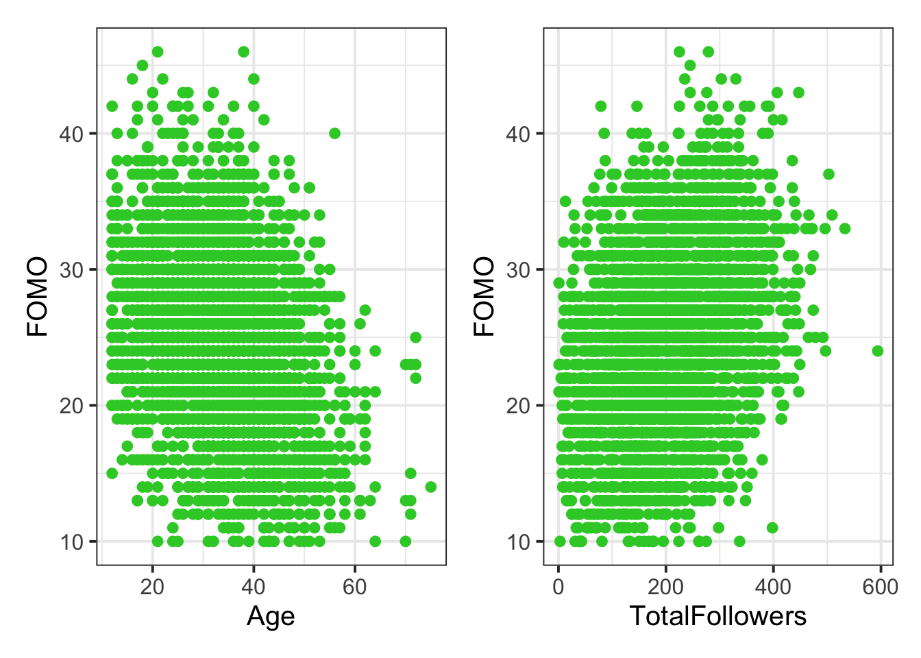
- Bright neon colours are generally to be avoided in scientific plots because many people find them hard to look at.
- There’s no reason for both of these plots to have any particular colour, since typically we want to use colour to distinguish different variables or different values of the same variable.
For example:
Code
p_age <- fomo |>
    ggplot(aes(x = Age, y = FOMO)) +
    geom_point(colour="limegreen")
p_followers <- fomo |>
    ggplot(aes(x = TotalFollowers, y = FOMO)) +
    geom_point(colour="tomato")

p_age + p_followers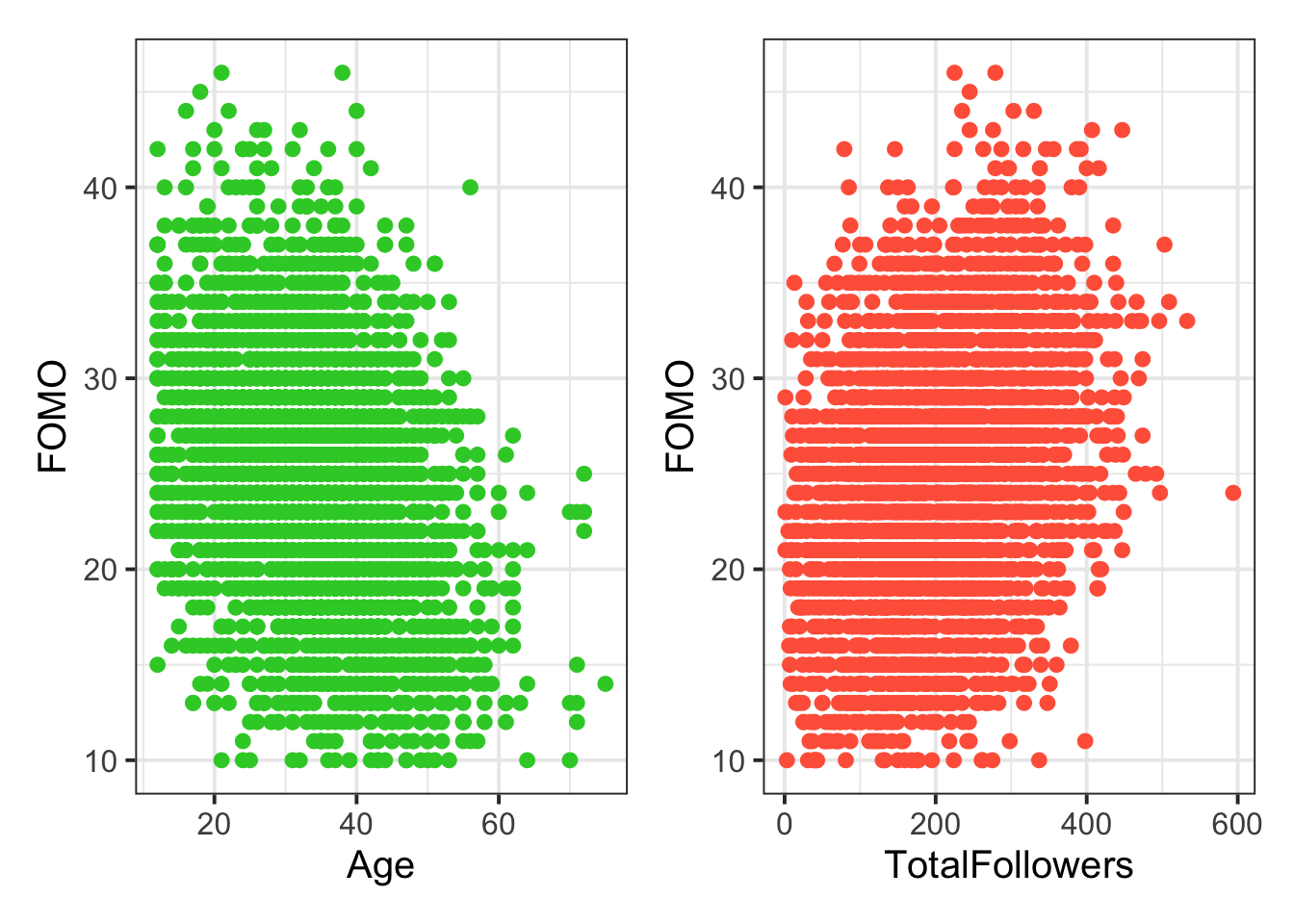
- Now we have different colours for each variable, which is fine, but these particular colours (green and red) are a problem for many people who are colourblind and cannot easily distinguish them. Here’s a link to a colourblind-friendly colour palette.
ImportantRepeating the same information in more than one place
For example, including both a plot like this and a table like the one below it:
Code
desc_FOMO <- ggplot(fomo, aes(y=FOMO))+
  geom_boxplot()
desc_Age <- ggplot(fomo, aes(y=Age))+
  geom_boxplot()

desc_FOMO + desc_Age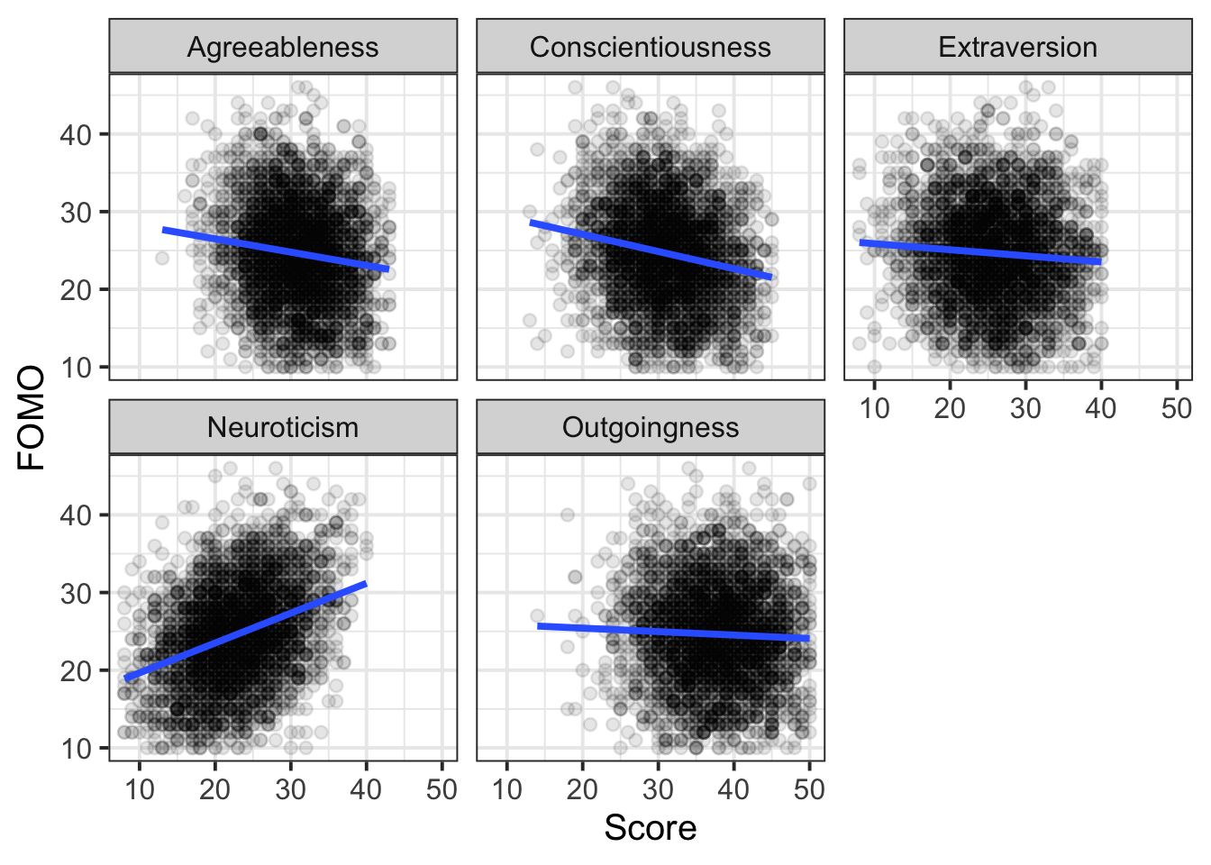
Code
desc_table <- fomo |>
    summarise(
        mean_Age=mean(Age),
        mean_FOMO=mean(FOMO),
        sd_Age=sd(Age),
        sd_FOMO=sd(FOMO),
        min_Age=min(Age),
        min_FOMO=min(FOMO),
        max_Age=max(Age),
        max_FOMO=max(FOMO)
    )
desc_table |> kable() |> kable_styling()| mean_Age | mean_FOMO | sd_Age | sd_FOMO | min_Age | min_FOMO | max_Age | max_FOMO |
|---|---|---|---|---|---|---|---|
| 33.61306 | 24.62849 | 10.41763 | 6.417429 | 12 | 10 | 75 | 46 |
- We get the same information from the plot and the table. Your precious space should be used only for one or the other (whichever you feel is easier for the reader to understand).
- The table also shows some issues with rounding, which we’ll mention as well the next box down.
ImportantRounding issues
For example:
results <- summary(m1)
results$coefficients |> kable() |> kable_styling()| Estimate | Std. Error | t value | Pr(>|t|) | |
|---|---|---|---|---|
| (Intercept) | 26.5219663 | 0.4460210 | 59.46350 | 0 |
| Age | -0.1651106 | 0.0098715 | -16.72603 | 0 |
| TotalFollowers | 0.0179895 | 0.0011009 | 16.34121 | 0 |
- It’s hard to correctly read numbers that contain a lot of decimal values, so it’s best to round all your numbers to two decimal places (or three places for p-values).
- Also, the p-value column rounds everything to 0—sort of the opposite problem, and also definitely not what we want!
- In this case, a better alternative to
results$coefficients |> kable()would probably be to manually create a data frame that contains the numbers you want to display.
ImportantHard-to-read “academic” writing style
For example:
In the present study, an analysis was undertaken to examine the association between individuals’ Fear of Missing Out (FOMO), the age of these individuals, and the quantity of followers that they possess on Instagram. It was predicted that the occurrence of an increase in age would be accompanied by the observation of a reduction in FOMO. Additionally, the prediction was made that an increase in the number of followers would occur alongside the observation of an increase in FOMO.
- Please, we beg, don’t worry about “sounding academic”! The more naturally you write, the easier it will be for your reader to understand you.
- It’s okay (even good!) to write sentences that use “we” or “I” and that describe the actions you took.
- Compare the writing above to easier-to-understand sentences like the following:
- “In this study, we wanted to find out how FOMO is associated with people’s age and how many followers they have on Instagram.”
- “We predicted that as age increases, FOMO will decrease.”
ImportantDrawing over-confident conclusions
For example:
The predictions were correct.
The hypothesis was verified.
Our research question was confirmed.
- Statistics cannot tell us whether things are correct or verified or confirmed.
- The best we can do, for a prediction, is tell whether it’s supported or not.
- And for hypotheses, we can only ever reject the null hypothesis; we never accept or verify the alternative hypothesis.
- And our research question just is. We don’t confirm it or reject it, we just do our best to address it.
Bonus challenge: RQ2
RQ: Do the Big 5 personality traits significantly predict FOMO, in addition to the effects of age and total Instagram followers?
TipProvided analysis code for RQ2
This code should resemble the analysis developed during lectures this week.
## Phase 1: Before model fitting ----

### 1a: Set up code and data – DONE ----

### 1b: Set up the variables we'll model ----

# RQ: Do the Big 5 personality traits significantly predict FOMO, in addition to the effects of age and total Instagram followers?

# Based on RQ, identify outcome variables and predictors.
# - Outcome: `FOMO`
# - Predictors: `Age`, `TotalFollowers`, and each OCEAN variable

# Based on RQ, decide whether to test hypotheses using coefficient significance tests or model comparison.
# - The RQ asks whether multiple predictors predict an outcome jointly, so it's a model comparison question.

# Set up continuous predictors. (e.g., any transformations?)
# - One option might be to z-score the OCEAN variables.
#   Zero is not very meaningful as-is.
#   But we actually don't care about interpreting any of those coefficients, just whether their inclusion helps the model.
#   So we can leave the OCEAN variables as-is too.
#   (Emphasise: this is a choice that could be made either way – just justify it!)

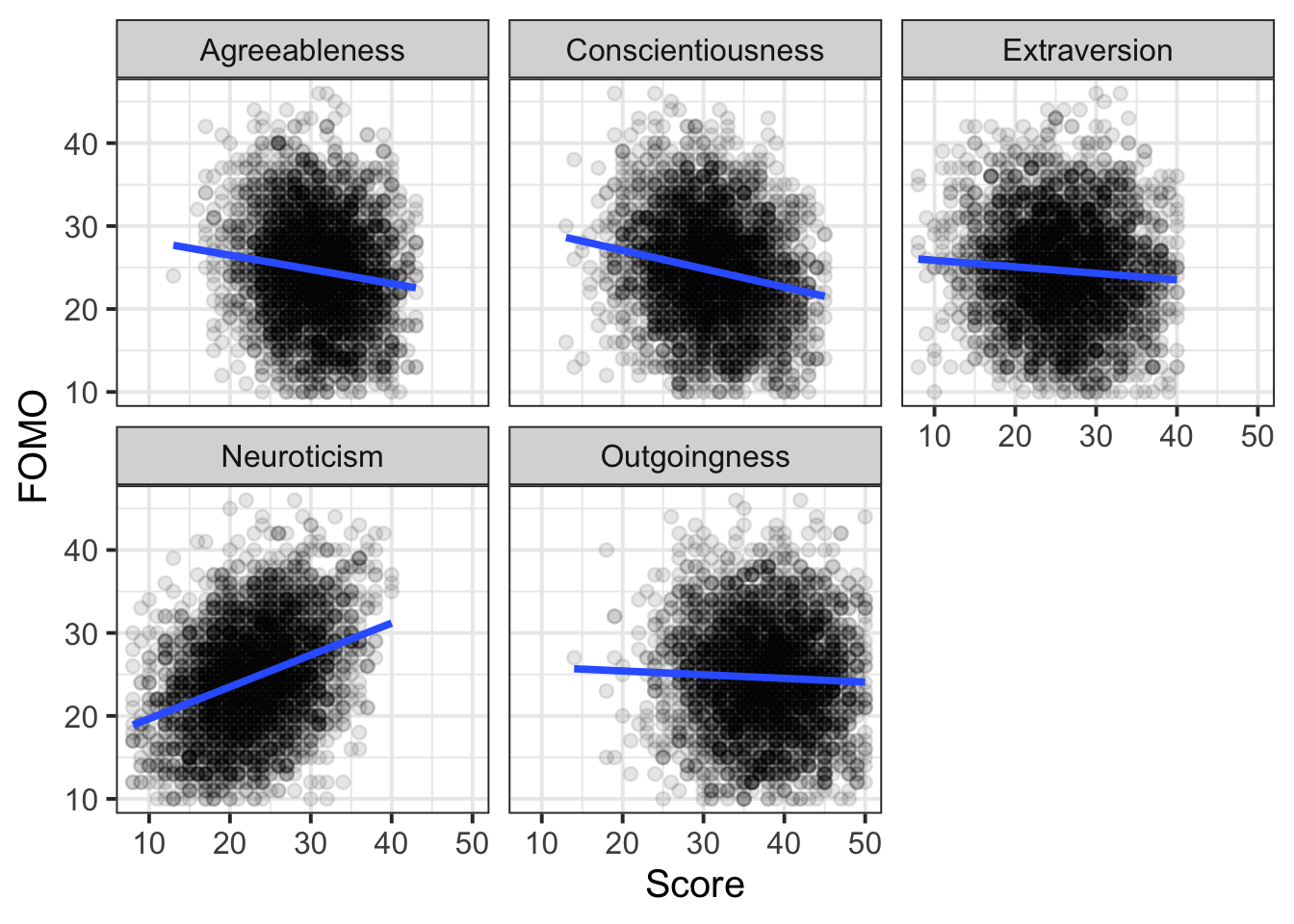
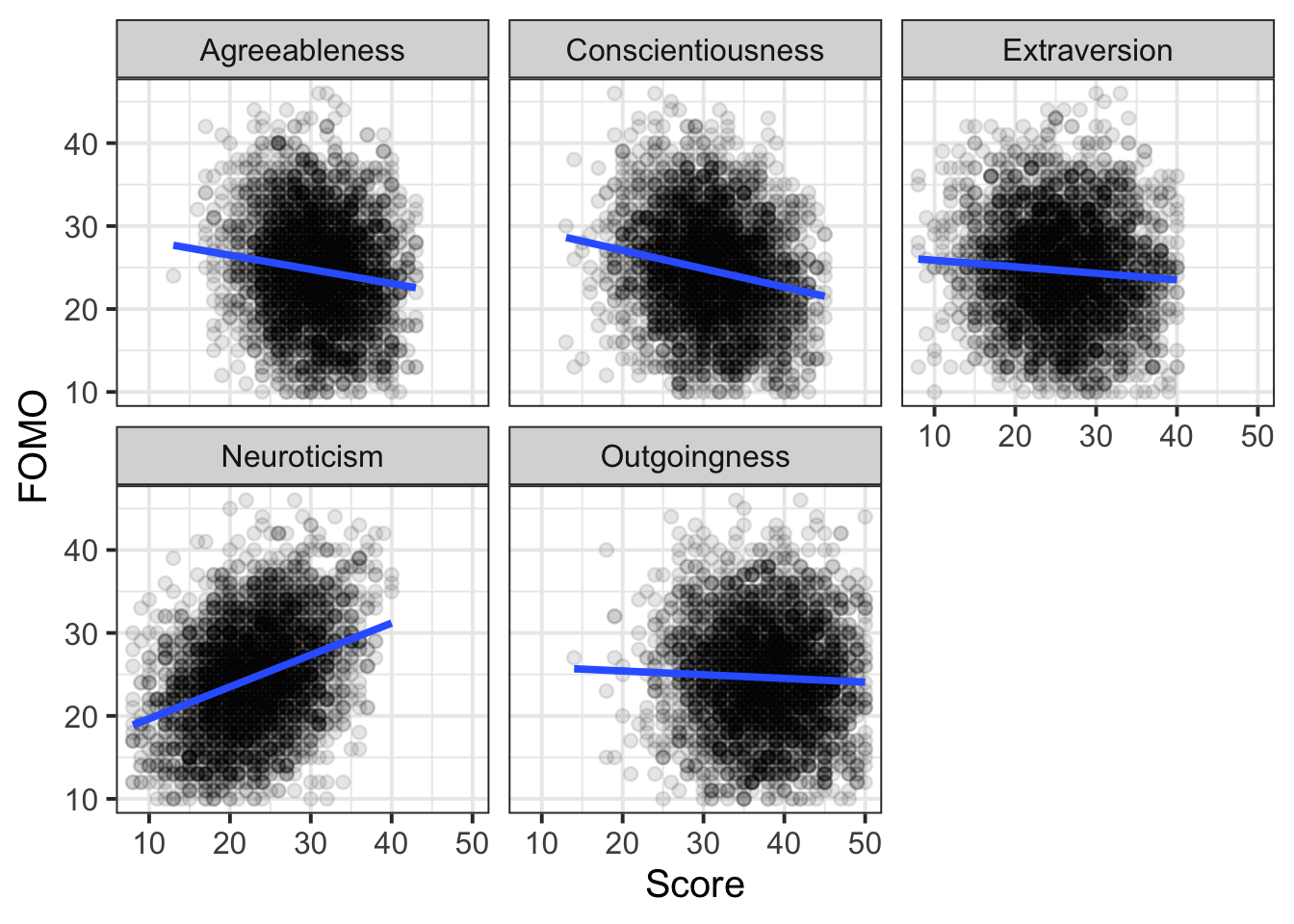
# Explore patterns in the data by plotting outcome and predictor variables together.
# - you could accomplish the same thing by making five plots and patchworking
#   them together, but this is a bit less repetitive

fomo |>
  rename(
    "Outgoingness" = O,
    "Conscientiousness" = C,
    "Extraversion" = E,
    "Agreeableness" = A,
    "Neuroticism" = N
  ) |>
  pivot_longer(
    cols = Neuroticism:Conscientiousness,
    names_to = 'Trait',
    values_to = 'Score'
  ) |>
  ggplot(aes(x = Score, y = FOMO)) +
  geom_point(alpha = 0.1) +
  geom_smooth(method = 'lm', se = F) +
  facet_wrap(~ Trait)

## Phase 2: Model fitting ----

# Write the mathematical model formulation for your model(s).
# - First model = model from RQ1. Second model:
#   $$
#     \text{FOMO} = \beta_0 +
#     (\beta_1 \cdot \text{Age}) +
#     (\beta_2 \cdot \text{Followers}) +
#     (\beta_3 \cdot \text{O}) +
#     (\beta_4 \cdot \text{C}) +
#     (\beta_5 \cdot \text{E}) +
#     (\beta_6 \cdot \text{A}) +
#     (\beta_7 \cdot \text{N}) +
#     \epsilon
#   $$

# Explicitly define the hypotheses that your RQ is aiming to test.
# - The null hypothesis that corresponds to this model comparison is that none of Big 5 predictors are significantly associated with FOMO.
#   $$
#   \begin{align}
#   H_0 &: \text{ All } \beta_j = 0 \text{ for } j = 3, 4, 5, 6, 7 \\
#   H_1 &: \text{ Any } \beta_j \neq 0 \\
#   \end{align}
#   $$

# Fit your model(s) using lm().
m2 <- lm(
  FOMO ~ Age + TotalFollowers + O + C + E + A + N,
  data = fomo
)

## Phase 3: After model fitting ----

### 3a: Plot and interpret model estimates ----

# Compare models and interpret model comparison statistics (if appropriate for your RQ).
# - Because these models are nested, we can use the incremental F-test via the `anova()` function.
anova(m1, m2)
Question 6
Set the scene (so the reader knows what you’re talking about).
Question 7
Describe and show the sample data (so that the reader knows how generalisable your analysis might be).
Question 8
Visualise and summarise data patterns that address the RQ (so the reader knows the basic pattern of what you found).
-
- Tip: If you transform any continuous predictors for analysis, use the transformed version of the predictor in the plot.
- Tip: Academic writing styles vary, but Elizabeth likes it when figure captions give the reader a brief take-home message about what they should see in the plot.
-
- Tip: If you find yourself listing loads of numbers in the text, consider using tables or plots instead (and they’re better for your word count too!).
- Tip: No inferential stats have been done yet, so we can’t make any claims just yet about whether the predictions were supported. But it is OK to say whether the results appear broadly in line with the prediction.
Question 9
Introduce your statistical analysis (so the reader can interpret the numbers you will report).
Question 10
Report the results of your analysis (so the reader knows exactly what you found).
-
- Tip: You don’t need to report every single parameter estimate. Focus on the one(s) you identified as being relevant to your prediction(s).
- Tip: Briefly link the direction and significance of the effect back to your earlier predictions—is the prediction supported by the parameter estimate?
Optional: Knit your report to PDF
Note: During the labs, please spend your time on the exercises above, not on rendering your document. This guidance is here in case you have extra time at the end.
Rmarkdown is a useful format because it can be used as a foundation for generating different kinds of documents. For the group report, you’ll be asked to render your Rmd file to PDF. Why not practice now?
First, make sure you have tinytex installed in R. This is what lets you convert things into PDF format.
Run the following code to install tinytex (you’ll only need to run it once).
install.packages("tinytex")
tinytex::install_tinytex()
Then ensure that the “yaml” (rhymes with “mammal”) header—the bit at the top of your Rmd document—looks something like this:
---
title: "this is my report title"
author: "B1234506"
date: "07/09/2025"
output: bookdown::pdf_document2
---
Then follow the instructions from the Rmd bootcamp to knit your Rmd document to PDF.
If you encounter errors, refer to the DAPR1 formatting resources / knitting checklist.
TipWhat to do if you cannot knit to PDF
If you are having issues knitting directly to PDF, try the following:
- Knit to HTML file
- Open your HTML in a web-browser (e.g. Chrome, Firefox)
- Print to PDF (Ctrl+P, then choose to save to PDF)
- Open file to check formatting
TipHiding code and/or output from code chunks
Review Lesson 5 of the rmd bootcamp for a detailed description/worked examples.
Hiding R Code
To not show the code of an R code chunk, and only show the output, write:
```{r, echo=FALSE}
# code goes here
```
Hiding R Output:
To show the code of an R code chunk, but hide the output, write:
```{r, results='hide'}
# code goes here
```
Hiding R code AND output
To hide both code and output of an R code chunk, write:
```{r, include=FALSE}
# code goes here
```