01: Simple linear regression

This week, you’ll use R to fit your first linear model, discover a few ways to extract information from it, and use it to generate predictions.

Get set up

Open RStudio.
Create a new .Rmd file for this week’s exercises.
Save it somewhere you can find it again.
Give it a clear name (for example, dapr2_lab01.Rmd).
In the first code chunk, use the library() function to load the packages you’ll need this week:
- tidyverse
- broom

If you don’t have these packages installed, then in the RStudio console (bottom left of the RStudio window), run the following code:

install.packages(c('tidyverse', 'broom'))

Research question (RQ): Does the number of weekly social interactions influence people’s wellbeing?

Data dictionary:

variable	description
age	Age in years of respondent
outdoor_time	Self report estimated number of hours per week spent outdoors
social_int	Self report estimated number of social interactions per week (both online and in-person)
routine	Binary 1=Yes/0=No response to the question 'Do you follow a daily routine throughout the week?'
wellbeing	Warwick-Edinburgh Mental Wellbeing Scale (WEMWBS), a self-report measure of mental health and wellbeing. The scale is scored by summing responses to each item, with items answered on a 1 to 5 Likert scale. The minimum scale score is 14 and the maximum is 70
location	Location of primary residence (City, Suburb, Rural)
steps_k	Average weekly number of steps in thousands (as given by activity tracker if available)

More detail about this dataset

From the Edinburgh & Lothians, 100 city/suburb residences and 100 rural residences were chosen at random and contacted to participate in the study. The Warwick-Edinburgh Mental Wellbeing Scale (WEMWBS) was used to measure mental health and wellbeing.

Participants filled out a questionnaire including items concerning: estimated average number of hours spent outdoors each week, estimated average number of social interactions each week (whether on-line or in-person), whether a daily routine is followed (yes/no). For those respondents who had an activity tracker app or smart watch, they were asked to provide their average weekly number of steps.

Read in and explore data

Question 1

Use the tidyverse function read_csv() to read in the data from https://uoepsy.github.io/data/wellbeing_rural.csv.

Store the data in a variable named mwdata (“mw” stands for “mental wellbeing”).

Code hint

Here’s the basic usage of read_csv() and how you can assign its output to a variable named mwdata.

Replace the ... with the actual location of the data.

mwdata <- read_csv("...")

Question 2

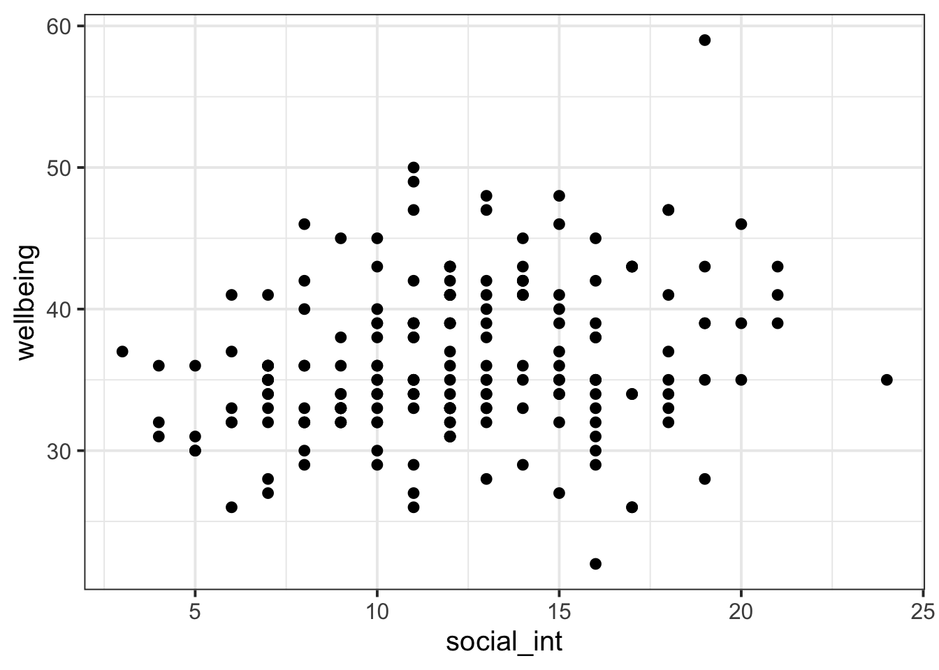
Our research question (RQ) is about how the number of social interactions per week might be associated with people’s wellbeing.

The relevant variables for this question are social_int and wellbeing.

Use ggplot to make a scatterplot that displays these two variables in relation to one another. Show social_int on the x axis (because it’s the independent variable) and wellbeing on the y axis (because it’s the dependent variable).

Code hint

Replace the ... with the appropriate variable or column names.

mwdata |>
  ggplot(aes(x = ..., y = ...)) +
  geom_point()

Set up and fit linear model

Question 3

Write the mathematical model formulation for a simple linear model with wellbeing as the outcome variable (i.e., dependent variable) and social_int as the one predictor variable (i.e., independent variable).

Here’s how to write the key symbols in Markdown so that they are rendered nicely as mathematical symbols:

$\beta_1$: write $\beta_1$
$\epsilon$: write $\epsilon$
$\cdot$ (multiplication symbol): write $\cdot$
To write variable names as regular text inside the $$ math mode notation, make sure to use the command $\text{...}$ .
To stop the underscore in social_int from causing problems, write social\_int instead (placing a backslash in front of the underscore).

🗂️ See Simple regression > Model specification flash card.

\[\text{wellbeing} = \beta_0 + (\beta_1 \cdot \text{social\_int}) + \epsilon\]

Write:

$$
\text{wellbeing} = \beta_0 + (\beta_1 \cdot \text{social\_int}) + \epsilon
$$

Question 4

Use the function lm() to fit a linear model which predicts wellbeing as a function of social_int. Name the result mdl.

🗂️ See Simple regression > Model building flash card.

Question 5

R offers many different ways to obtain the coefficient estimates from a fitted model. Run each of the following lines of code and see what each one does. Which one gives you the most information?

mdl
mdl$coefficients
coef(mdl)
coefficients(mdl)
summary(mdl)

Question 6

Take the intercept and slope coefficients estimated in mdl, round them both to two decimal points, and substitute them appropriately into the mathematical model expression you wrote in Q3.

🗂️ See Simple regression > Model building flash card.

coef(mdl) |> round(2)

(Intercept)  social_int 
      32.41        0.32

Rounded to two decimal points, the intercept is 32.41, and the slope over social_int is 0.32.

The intercept corresponds to $\beta_0$ and the slope corresponds to $\beta_1$. So we will replace $\beta_0$ with 32.41 and $\beta_1$ with 0.32:

\[ \text{wellbeing} = 32.41 + (0.32 \cdot \text{social\_int}) + \epsilon \]

Write:

$$
\text{wellbeing} = 32.41 + (0.32 \cdot \text{social\_int}) + \epsilon
$$

Question 7

In the context of this data and RQ, write one sentence interpreting what the intercept means and one sentence interpreting what the slope over social_int means.

🗂️ See Simple regression > Interpreting results flash card.

Use linear model to make predictions

Question 8

The third row of mwdata represents somebody with 11 social interactions per week:

mwdata[3,]

# A tibble: 1 x 7
    age outdoor_time social_int routine wellbeing location steps_k
  <dbl>        <dbl>      <dbl>   <dbl>     <dbl> <chr>      <dbl>
1    25           19         11       1        35 rural       49.8

Calculate the wellbeing score that the model would estimate for this person with social_int = 11.

To do this:

Take the mathematical model expression you wrote for Q6,
remove the $+ \epsilon$ bit (why? because model predictions correspond to the exact line the model has estimated, so we don’t want to include the error/residual term),
substitute the value 11 for the variable $\text{social\_int}$,
and conduct the multiplication and addition as defined by the mathematical expression. (Remember that you can use the console in RStudio as a calculator.)

🗂️ See Compute model-predicted values > Example flash card.

\[ \begin{align} \text{wellbeing}_{\text{social\_int} = 11} &= 32.41 + (0.32 \cdot \text{social\_int}) \\ &= 32.41 + (0.32 \cdot 11) \\ &= 32.41 + 3.52 \\ &= 35.93 \\ \end{align} \]

Write:

$$
\begin{align}
\text{wellbeing}_{\text{social\_int} = 11} &= 32.41 + (0.32 \cdot \text{social\_int}) \\
  &= 32.41 + (0.32 \cdot 11) \\
  &= 32.41 + 3.52 \\
  &= 35.93 \\
\end{align}
$$

Question 9

Now you’ll try out a new function called augment(). It comes from the package broom, and it is very useful for computing predictions from linear models.

Run the following code:

augment(mdl)

You should see a data frame with a bunch of columns. For now, we are only interested in the first four:

wellbeing: the observed wellbeing values we gave to the model
social_int: the observed social_int values we gave to the model
.fitted: the predicted outcome values from the model (“fitted” or model-fitted” is another way to say “predicted”)
.resid: the residuals, that is, the difference between each predicted value and each actual observed values

Look at the third row of this data frame. Does the value in the .fitted column match the value you calculated above in Q8?

🗂️ See Compute model-predicted values > For sample data flash card.

The Piazza forum

Question 10

Finally: we want you to get familiar with the course’s Piazza page.

Access Piazza from Learn > Quick links > Piazza Q&A.

Piazza is a discussion forum where you can anonymously post questions that your coursemates and instructors can see and respond to. Please use Piazza to ask us your questions!

Asking on Piazza is better than asking by email because on Piazza, everybody can benefit from your questions. And if you have a question, you certainly won’t be the only one.

Your final task this week is to get to know Piazza by navigating to Elizabeth’s post called “Lab 01: Something nice from this summer” and replying (anonymously or not, as you prefer) with something nice that YOU experienced this summer.

(Note: we may switch Q&A systems partway through the year, because the uni might be changing from Piazza to something new. We’ll keep you posted!)