| variable | description |
|---|---|
| treatment | which one of four treatment conditions the participant was assigned - control (water), coffee, mint tea, or red bull |
| wpm | average number of words typed per minute |
06: Treatment coding
This week, you’ll practice implementing and interpreting a treatment-coded categorical predictor with four levels.
NoteGet set up
- Open RStudio.
- Create a new .Rmd file for this week’s exercises.
- Save it somewhere you can find it again.
- Give it a clear name (for example,
dapr2_lab06.Rmd). - In the first code chunk, load the packages you’ll need this week (and install them if you don’t have them already):
tidyverse
To investigate if typing speed, measured in words per minute (WPM), differs between people who’ve consumed different kinds of beverages, the researchers conducted an experiment where 40 participants were each randomly allocated to one of four beverage conditions.
The data in caffeinedrink.csv contained two attributes collected from \(n=40\) participants:
Get to know the data
Question 1
Read in the data from https://uoepsy.github.io/data/caffeinedrink.csv and store it in a variable named wpm_data.
Question 2
As you know, a quick-and-dirty way to plot a numeric outcome as a function of a categorical predictor is a boxplot:
wpm_data |>
  ggplot(aes(x = treatment, y = wpm)) +
  geom_boxplot()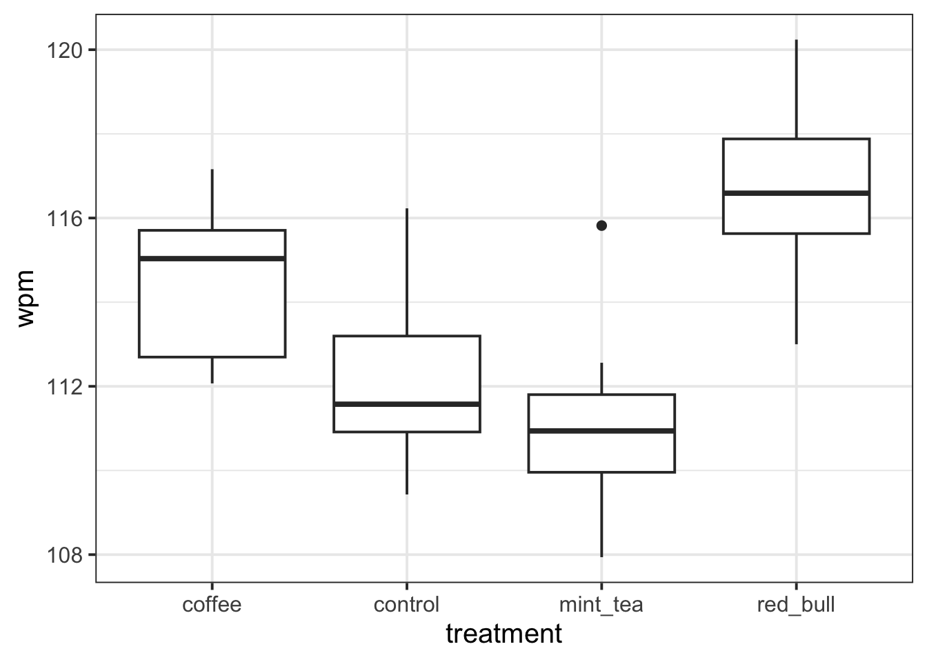
But by summarising the data into median and inter-quartile range, you don’t actually see the information that’s helpful for linear modelling, where we care about group means, not medians. (And sometimes the distribution of data is just totally misrepresented; read more here if you’re curious).
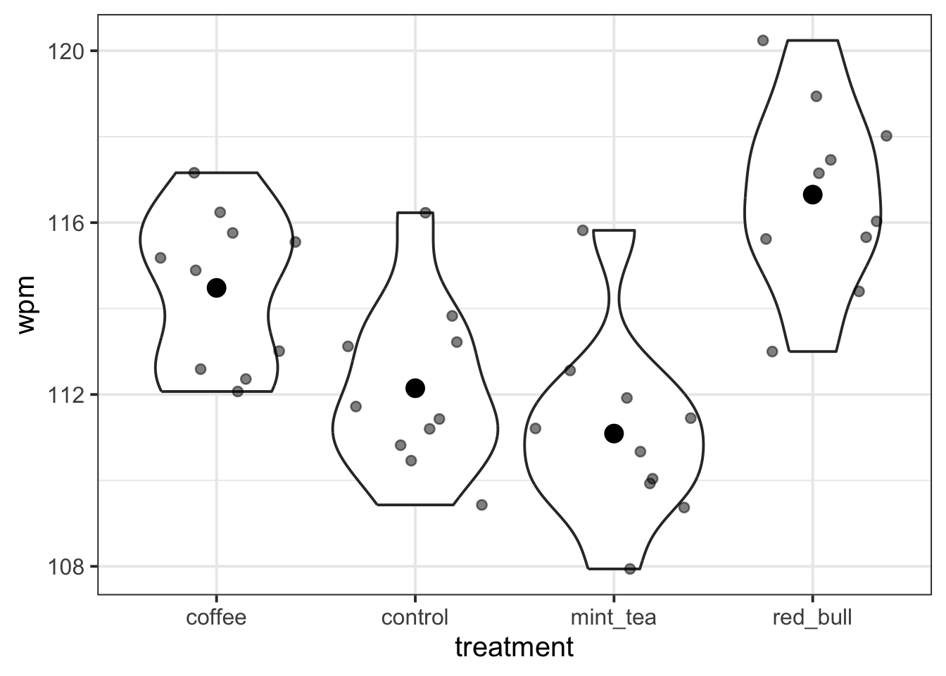
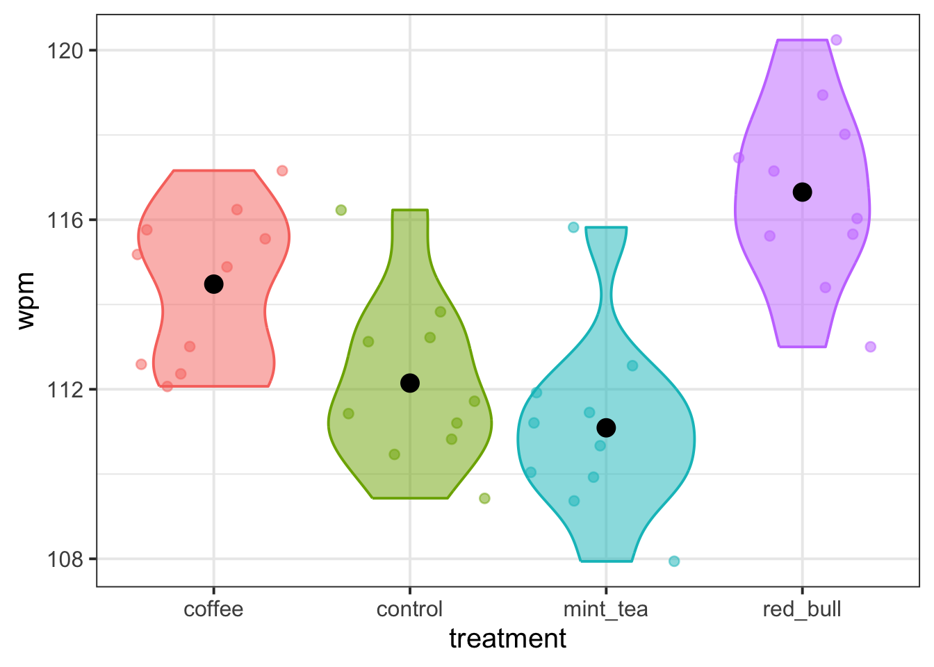
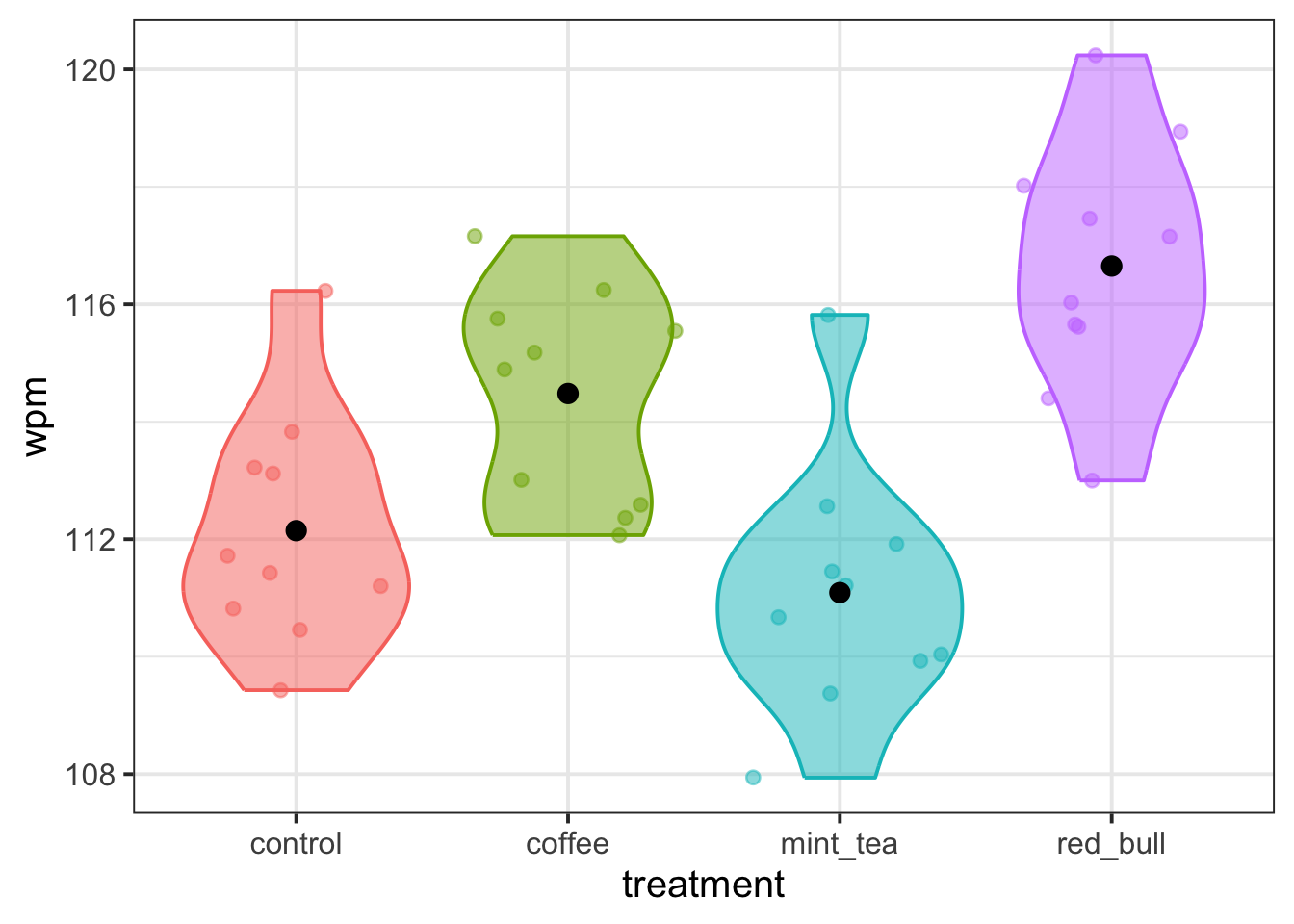
Elizabeth’s favourite alternative is the violin plot (a kind of vertical density plot, which shows the lumps and bumps of the data’s distribution more faithfully) with jittered points over top (so that we can see each actual observed data point), and with each group’s mean shown as a big black dot.
To make a violin plot that shows how wpm varies based on beverage treatment, copy the following code template, replace the ... bits with the appropriate variable names, and create your own violin plot.
... |>
  ggplot(aes(x = ..., y = ...)) +
  geom_violin() +
  geom_jitter(height = 0, alpha = 0.5) +
  stat_summary(fun = mean, geom = 'point', size = 4)
(Once you have this code running, if you’re not sure what part of it does, then comment out (that is, put a hashtag # at the start of the line) or delete that bit, try running what’s left over, and see what changes.)
🗂️ See Exploring data visually > Violin plot flash card.
Think about treatment coding
Question 3
Which of the four levels of treatment do you think would be a suitable reference level? Write down which level you’d choose, and write one sentence to describe why you chose that one.
🗂️ See Treatment coding flash card.
Question 4
Based on the reference level you chose above, you’ll now try to predict what the contrast matrix for the treatment variable will look like. (You’ll get R to generate the actual contrast matrix later, and you can check your predictions then.)
Here is some code for creating a Markdown table. Copy this code to your own Rmd file, placing it outside a code chunk (in other words: treat it as if it’s text, not R code).
|            | ... | ... | ... |
| ---------- | --- | --- | --- |
| `coffee`   | ... | ... | ... |
| `control`  | ... | ... | ... |
| `mint_tea` | ... | ... | ... |
| `red_bull` | ... | ... | ... |
Your task is to replace all the ... bits in this table with appropriate values.
Specifically, fill in the column names with the appropriate levels of treatment, and fill in the other empty cells with 0s and 1s.
🗂️ See Treatment coding > Three-level predictor flash card.
Question 5
Now you’ll check your work from the previous question.
Using mutate(), convert treatment into a factor and reorder the levels so that your chosen reference level comes first.
🗂️ See Treatment coding > Changing reference level flash card.
Then, run the following code to produce the contrast matrix:
contrasts(wpm_data$treatment)Check: Did your predictions match this output? (Don’t worry if the rows are in a different order! Just pay attention to the column names and where the 0s and 1s are placed.)
Set up the model
Question 6
Write the mathematical model formulation for the model that we’re about to fit, using the dummy variables from the contrast matrix generated by R in Q5.
🗂️ See Treatment coding > Mathematical model formulation flash card.
Question 7
The model you’ll fit will have four coefficients: one intercept and three slopes which each compare one of the non-reference levels back to the reference level.
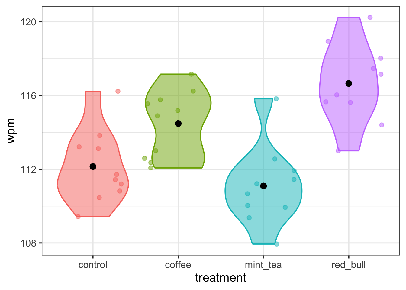
Based on the plot you created back in Q2, write down your best guess about the approximate value that each of the model’s four coefficients will have.
If you’re really not sure, at least write down whether you think each coefficient will be positive or negative.
After you fit the model, you’ll check your predictions. (I know this is a hard task, but I promise that making these predictions will help your understanding in the long run.)
🗂️ See Treatment coding > Model fit and interpretation flash card.
Question 8
Now fit the model in R and display the model summary.
Check: Were your predictions about the coefficients correct?
If they were, celebrate! If not, try to figure out how you can update your thinking to better match the results (and ask a tutor/ask on Piazza if you’re not sure!).
🗂️ See Treatment coding > Model fit and interpretation flash card.
A new reference level
Question 9
For these last two questions, imagine changing the reference level to coffee (or if you already used coffee as your reference level, imagine changing it to something else).
If the reference level were updated to coffee, what would the model’s coefficients be estimating?
Using the plot again, visually estimate the approximate value (or at least the sign: positive or negative) of all four model coefficients.
🗂️ See Treatment coding > Model fit and interpretation flash card.
Question 10
Now you’ll actually be changing the reference level and seeing what else changes. For this whole question, we recommend copying and pasting your code from earlier and just modifying the relevant bits of it—that way you don’t have to retype everything!
First: change the reference level of treatment to coffee (or if you already used coffee as your reference level, change it to something else).
Next, generate the contrast matrix to verify your new reference level.
🗂️ See Treatment coding > Changing reference level flash card.
Then re-fit the model and display the model summary.
🗂️ See Treatment coding > Model fit and interpretation flash card.
Check: Were your predictions from Q9 supported? Why or why not?
Optional but recommended (your future self will thank you!): After checking your predictions, write a little guide for yourself, in your own words, about how to interpret treatment-coded predictors.
Optional: Knit your report to PDF
Note: During the labs, please spend your time on the exercises above, not on rendering your document. This guidance is here in case you have extra time at the end.
Rmarkdown is a useful format because it can be used as a foundation for generating different kinds of documents. For the group report, you’ll be asked to render your Rmd file to PDF. Why not practice now?
First, make sure you have tinytex installed in R. This is what lets you convert things into PDF format.
Run the following code to install tinytex (you’ll only need to run it once).
install.packages("tinytex")
tinytex::install_tinytex()
Then ensure that the “yaml” (rhymes with “mammal”) header—the bit at the top of your Rmd document—looks something like this:
---
title: "this is my report title"
author: "B1234506"
date: "07/09/2025"
output: bookdown::pdf_document2
---
Then follow the instructions from the Rmd bootcamp to knit your Rmd document to PDF.
If you encounter errors, refer to the DAPR1 formatting resources / knitting checklist.
TipWhat to do if you cannot knit to PDF
If you are having issues knitting directly to PDF, try the following:
- Knit to HTML file
- Open your HTML in a web-browser (e.g. Chrome, Firefox)
- Print to PDF (Ctrl+P, then choose to save to PDF)
- Open file to check formatting
TipHiding code and/or output from code chunks
Review Lesson 5 of the rmd bootcamp for a detailed description/worked examples.
Hiding R Code
To not show the code of an R code chunk, and only show the output, write:
```{r, echo=FALSE}
# code goes here
```
Hiding R Output:
To show the code of an R code chunk, but hide the output, write:
```{r, results='hide'}
# code goes here
```
Hiding R code AND output
To hide both code and output of an R code chunk, write:
```{r, include=FALSE}
# code goes here
```