Section B: Weeks 6-9 Recap
In the second part of the lab, there is no new content - the purpose of the recap section is for you to revisit and revise the concepts you have learned over the last 4 weeks.
Before you expand each of the boxes below, think about how comfortable you feel with each concept.
Errors and Power in Hypothesis Testing
When testing a hypothesis, we reach one of the following two decisions:
- failing to reject \(H_0\) as the evidence against it is not sufficient
- rejecting \(H_0\) as we have enough evidence against it
However, irrespective of our decision, the underlying truth can either be that
-
\(H_0\) is actually false
-
\(H_0\) is actually true
Hence, we have four possible outcomes following a hypothesis test:
- We failed to reject \(H_0\) when it was true, meaning we made a Correct decision
- We rejected \(H_0\) when it was false, meaning we made a Correct decision
- We rejected \(H_0\) when it was true, committing a Type I error
- We failed to reject \(H_0\) when it was false, committing a Type II error
In the first two cases we are correct, while in the latter two we committed an error.
When we reject the null hypothesis, we never know if we were correct or committed a Type I error, however we can control the chance of us committing a Type I error.
Similarly, when we fail to reject the null hypothesis, we never know if we are correct or we committed a Type II error, but we can also control the chance of us committing a Type II error.
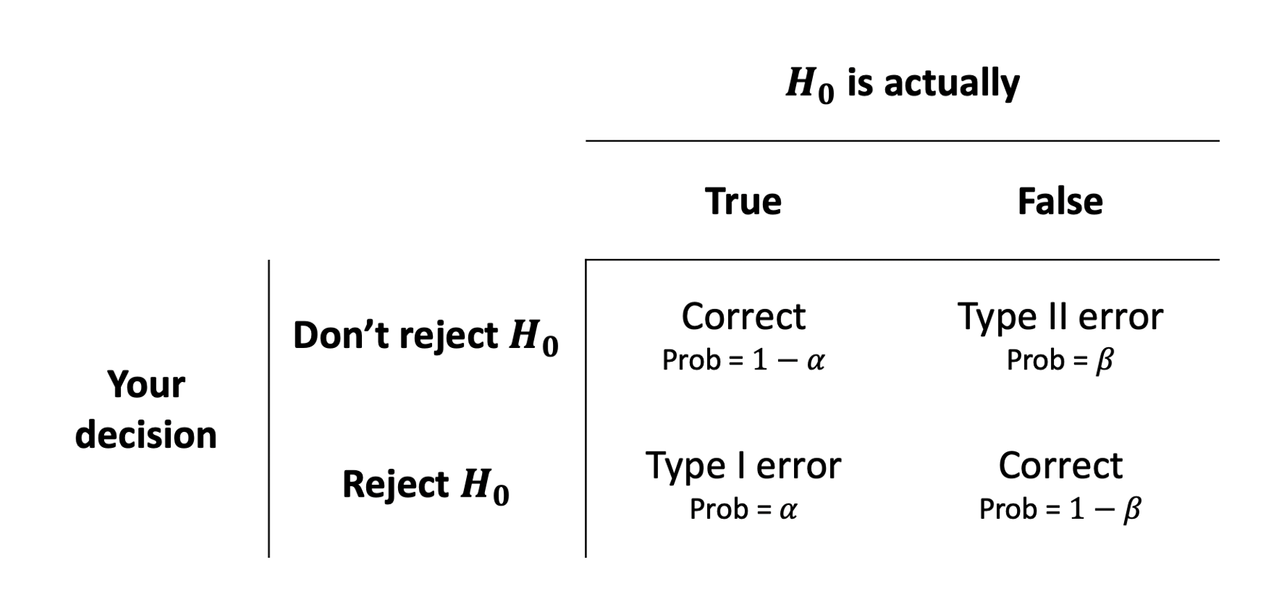
The following table summarises the two types of errors that we can commit:
A Type I error corresponds to a false discovery, while a type II error corresponds to a failed discovery/missed opportunity.
Each error has a corresponding probability:
- The probability of incorrectly rejecting a true null hypothesis is \(\alpha = P(\text{Type I error})\)
- The probability of incorrectly not rejecting a false null hypothesis is \(\beta = P(\text{Type II error})\)
A related quantity is Power, which is defined as the probability of correctly rejecting a false null hypothesis.
Power
Power is the probability of rejecting a false null hypothesis. That is, it is the probability that we will find an effect when it is in fact present. \[
\text{Power} = 1 - P(\text{Type II error}) = 1 - \beta
\]
See S2 Week 6 Lecture, and S2 Week 6 Lab for further details, examples, and to revise these concepts further.
Factors Affecting Power
In practice, it is ideal for studies to have high power while using a relatively small significance level such as .05 or .01. For a fixed \(\alpha\), the power increases in the same cases that P(Type II error) decreases, namely as the sample size increases and as the parameter value moves farther into the H values away from the H0 value.
The power of a test is affected by the following factors:
-
sample size. Power increases as the sample size increases.
-
effect size. Power increases as the parameter value moves farther into the \(H_1\) values away from the \(H_0\) value.
-
significance level. Power increases as the significance level increases.
Out of these, increasing the significance level \(\alpha\) is never an acceptable way to increase power as it leads to more Type I errors, i.e. a higher chance of incorrectly rejecting a true null hypothesis (false discoveries).
See S2 Week 6 Lecture, and S2 Week 6 Lab for further details, examples, and to revise these concepts further.
Effect Size
Effect size refers to the “detectability” of your alternative hypothesis. In simple terms, it compares the distance between the alternative and the null hypothesis to the variability in your data.
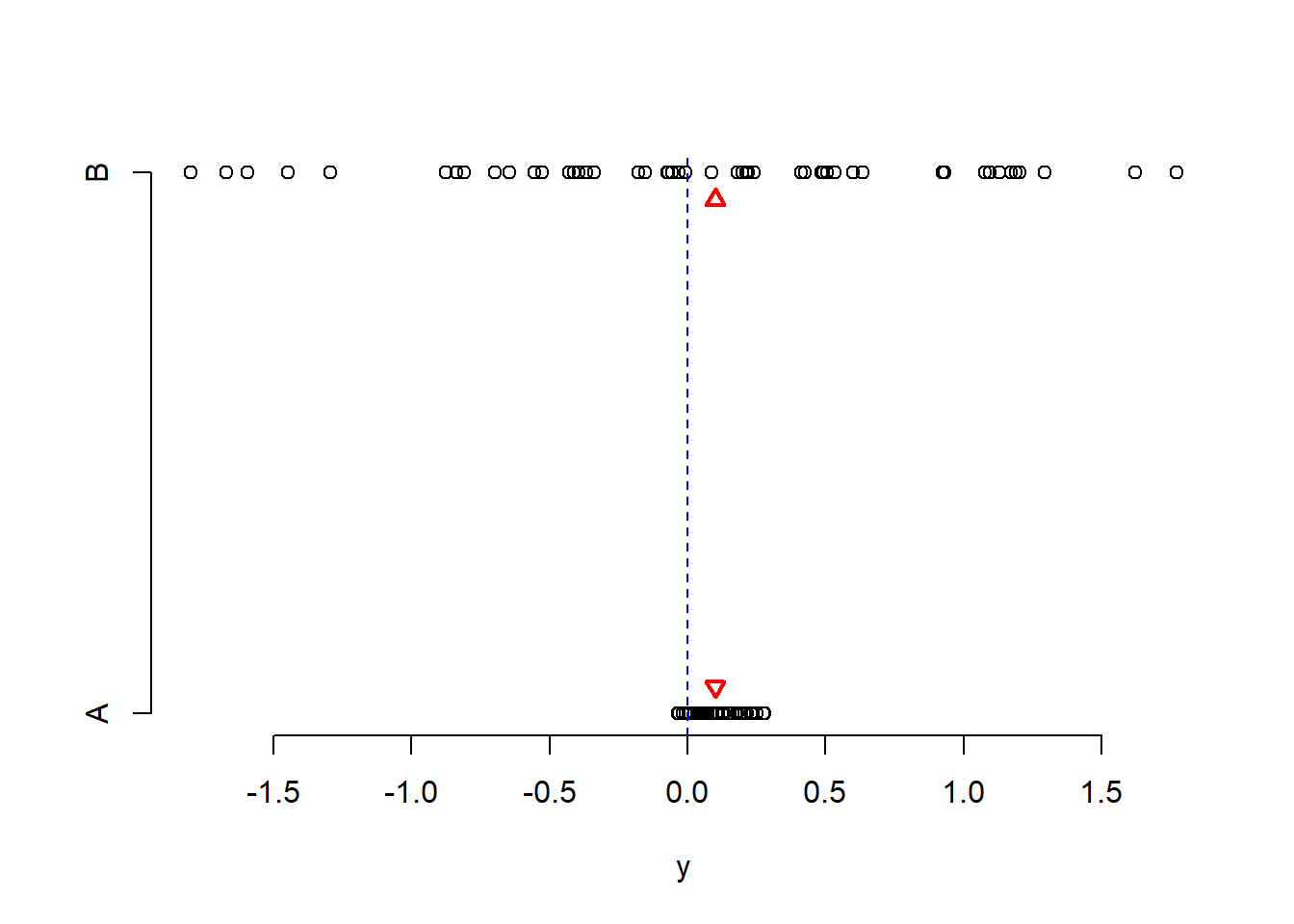
For simplicity consider comparing a mean: \(H_0: \mu = 0\) vs \(H_1: \mu \neq 0\). If the sample mean were really 0.1 and the null hypothesis is 0, the distance is 0.1 - 0 = 0.1.
Now, a distance of 0.1 has a different weight in the following two scenarios.
Scenario 1. Data vary between -1 and 1.
Scenario 2. Data vary between -1000 and 1000.
Clearly, in Scenario 1 a distance of of 0.1 is a big difference. Conversely, in Scenario 2 a distance of 0.1 is not an interesting difference, it’s negligible compared to the magnitude of the data.
See S2 Week 6 Lecture, and S2 Week 6 Lab for further details, examples, and to revise these concepts further.
The pwr Package
You will perform power analysis using the pwr package. To install it, run install.packages("pwr") in your console, then run library(pwr) in your RMarkdown file.
The following functions are available.
pwr.2p.test |
Two proportions (equal n) |
pwr.2p2n.test |
Two proportions (unequal n) |
pwr.anova.test |
Balanced one-way ANOVA |
pwr.chisq.test |
Chi-square test |
pwr.f2.test |
General linear model |
pwr.p.test |
Proportion (one sample) |
pwr.r.test |
Correlation |
pwr.t.test |
t-tests (one sample, two samples, paired) |
pwr.t2n.test |
t-test (two samples with unequal n) |
For each function, you can specify three of four arguments (sample size, alpha, effect size, power) and the fourth argument will be calculated for you.
Of the four quantities, effect size is often the most difficult to specify. Calculating effect size typically requires some experience with the measures involved and knowledge of past research.
Typically, specifying effect size requires you to read published literature or past papers on your research topic, to see what effect sizes were found and what significant results were reported. Other times, this might come from previous collected data or subject-knowledge from your colleagues.
But what can you do if you have no clue what effect size to expect in a given study? Cohen (1988) provided guidelines for what a small, medium, or large effect typically is in the behavioral sciences.
| t-test |
0.20 |
0.50 |
0.80 |
|
| ANOVA |
0.10 |
0.25 |
0.40 |
|
| Linear regression |
0.02 |
0.15 |
0.35 |
|
See S2 Week 6 Lecture, and S2 Week 6 Lab for further details, examples, and to revise these concepts further.
Power for t-tests
We compare the mean of a response variable between two groups using a t-test. For example, if you are comparing the mean response between two groups, say treatment and control, the null and alternative hypotheses are: \[
H_0 : \mu_t - \mu_c = 0
\]
\[
H_1 : \mu_t - \mu_c \neq 0
\]
The effect size in this case is Cohen’s \(D\): \[
D = \frac{(\bar x_t - \bar x_c) - 0}{s_p}
\] where
-
\(\bar x_t\) and \(\bar x_c\) are the sample means in the treatment and control groups, respectively
-
\(s_p\) is the “pooled” standard deviation
Cohen’s \(D\) measures the distance between (a) the observed difference in means from (b) the hypothesised value 0, and compares this to the variability in the data.
In R we use the function
pwr.t.test(n = , d = , sig.level = , power = , type = , alternative = )
where
-
n = the sample size
-
d = the effect size
-
sig.level = the significance level \(\alpha\) (the default is 0.05)
-
power = the power level.
-
type = the type of t-test to perform: either a two-sample t-test (“two.sample”), a one-sample t-test (“one.sample”), or a dependent sample t-test (“paired”). A two-sample test is the default.
-
alternative = whether the alternative hypothesis is two-sided (“two.sided”) or one-sided (“less” or “greater”). A two-sided test is the default.
See S2 Week 6 Lecture, and S2 Week 6 Lab for further details, examples, and to revise these concepts further.
Power for Linear Regression
In linear regression, the relevant function in R is:
where - u = numerator degrees of freedom - v = denominator degrees of freedom - f2 = effect size
Here you have one model,
\[
y = \beta_0 + \beta_1 x_1 + \dots + \beta_k x_k + \epsilon
\]
and you wish to find the minimum sample size required to answer the following test of hypothesis with a given power:
\[
\begin{aligned}
H_0 &: \beta_1 = \beta_2 = \dots = \beta_k = 0 \\
H_1 &: \text{At least one } \beta_i \neq 0 \\
\end{aligned}
\]
The appropriate formula for the effect size is:
\[
f^2 = \frac{R^2}{1 - R^2}
\]
And the numerator degrees of freedom are \(\texttt u = k\), the number of predictors in the model.
The denominator degrees of freedom returned by the function will give you:
\[
\texttt v = n - (k + 1) = n - k - 1 \\
\]
From which you can infer the sample size as
\[
n = \texttt v + k + 1 \\
\]
In this case you would have a smaller model \(m\) with \(k\) predictors and a larger model \(M\) with \(K\) predictors:
\[
\begin{aligned}
m &: \quad y = \beta_0 + \beta_1 x_1 + \dots + \beta_{k} x_k + \epsilon \\
M &: \quad y = \beta_0 + \beta_1 x_1 + \dots + \beta_{k} x_k
+ \underbrace{\beta_{k + 1} x_{k+1} + \dots + \beta_{K} x_K}_{\text{extra predictors}}
+ \epsilon \\
\end{aligned}
\]
This case is when you wish to find the minimum sample size required to answer the following test of hypothesis:
\[
\begin{aligned}
H_0 &: \beta_{k+1} = \beta_{k+2} = \dots = \beta_K = 0 \\
H_1 &: \text{At least one of the above } \beta \neq 0 \\
\end{aligned}
\]
You need to use the R-squared from the larger model \(R^2_M\) and the R-squared from the smaller model \(R^2_m\). The appropriate formula for the effect size is:
\[
f^2 = \frac{R^2_{M} - R^2_{m}}{1 - R^2_M}
\]
Here, the numerator degrees of freedom are the extra predictors: \(\texttt u = K - k\).
The denominator degrees of freedom returned by the function will give you (here you use \(K\) the number of all predictors in the larger model):
\[
\text v = n - (K + 1) = n - K - 1
\]
From which you can infer the sample size as
\[
n = \text v + K + 1
\]
See S2 Week 6 Lecture, and S2 Week 6 Lab for further details, examples, and to revise these concepts further.
Probability, Odds, Log-Odds
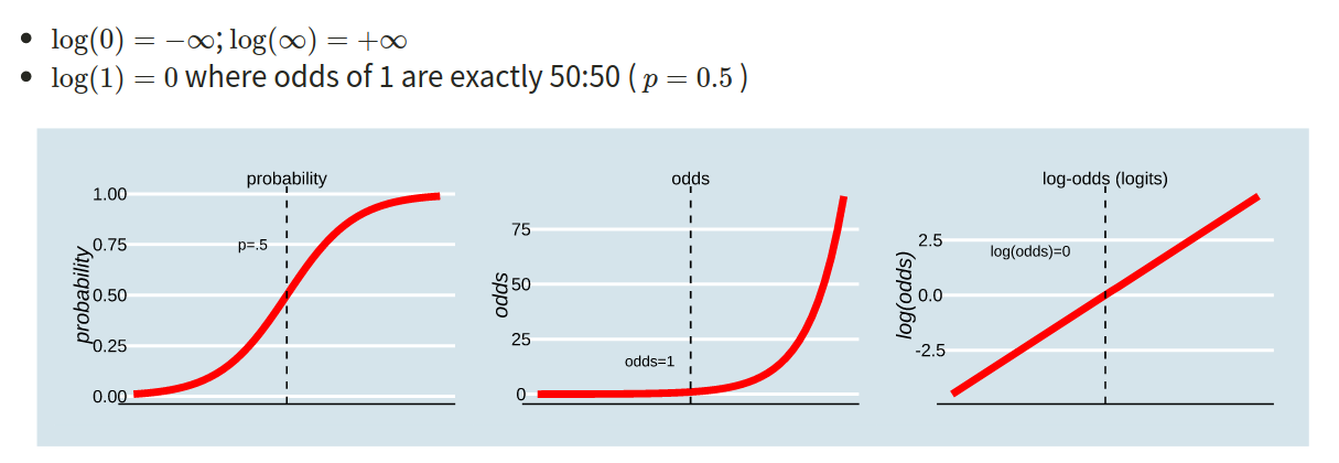
The probability \(p\) ranges from 0 to 1.
The odds \(\frac{p}{1-p}\) ranges from 0 to \(\infty\).
The log-odds \(\log \left( \frac{p}{1-p} \right)\) ranges from \(-\infty\) to \(\infty\).
In the labs, we used “log” to denote log-odds. In the lectures, you will have seen this denoted as “ln”.
In order to understand the connections among these concepts, lets work with an example where the probability of an event occurring is 0.2:
\[
\text{odds} = (\frac{0.2}{0.8}) = 0.25
\]
- Log-odds of the event occurring:
\[
log(\frac{0.2}{0.8}) = -1.3863 \\ \ \\
\]
OR
\[
log(0.25) = -1.3863
\]
- Probability can be reconstructed as:
\[
(\frac{odds}{1+odds}) = (\frac{0.25}{1+0.25}) = 0.2 \\ \ \\
\]
OR
\[
(\frac{exp(log(odds))}{1+exp(log(odds))}) = (\frac{exp(-1.3863)}{1+exp(-1.3683)}) = (\frac{0.25}{1.25}) = 0.2
\]
In R:
-
obtain the odds
odds <- 0.2 / (1 - 0.2)
-
obtain the log-odds for a given probability
log_odds <- log(0.25)
OR
log_odds <- qlogis(0.2)
-
obtain the probability from the odds
prob_O <- odds / (1 + odds)
-
obtain the probability from the log-odds
prob_LO <- exp(log_odds) / (1 + exp(log_odds))
OR
prob_LO <- plogis(log_odds)
Binary Logistic Regression
When a response (y) is binary coded (e.g., 0/1; failure/success; no/yes; fail/pass; unemployed/employed) we must use logistic regression. The predictors can either be continuous or categorical.
\[
{\log(\frac{p_i}{1-p_i})} = \beta_0 + \beta_1 \ x_{i1}
\]
In R:
glm(y ~ x1 + x2, data = data, family = binomial)
Interpretation of Coefficients
To interpret the fitted coefficients, we first exponentiate the model: \[
\begin{aligned}
\log \left( \frac{p_x}{1-p_x} \right) &= \beta_0 + \beta_1 x \\
e^{ \log \left( \frac{p_x}{1-p_x} \right) } &= e^{\beta_0 + \beta_1 x } \\
\frac{p_x}{1-p_x} &= e^{\beta_0} \ e^{\beta_1 x}
\end{aligned}
\]
and recall that the probability of success divided by the probability of failure is the odds of success. \[
\frac{p_x}{1-p_x} = \text{odds}
\]
Let’s apply this to an example where we are trying to determine whether the probability of having senility symptoms change as a function of Wechsler Adult Intelligence Scale (WAIS) score, where we fit the following model:
\[
\begin{aligned}
Model_{Senility}: \qquad \log \left( \frac{p}{1 - p}\right) = \beta_0 + \beta_1 \cdot \text{WAIS Score} + \epsilon
\end{aligned}
\]
Intercept
\[
\text{If }x = 0, \qquad \frac{p_0}{1-p_0} = e^{\beta_0} \ e^{\beta_1 x} = e^{\beta_0}
\]
That is, \(e^{\beta_0}\) represents the odds of having symptoms of senility for individuals with a WAIS score of 0.
In other words, for those with a WAIS score of 0, the probability of having senility symptoms is \(e^{\beta_0}\) times that of non having them.
Slope
\[
\text{If }x = 1, \qquad \frac{p_1}{1-p_1} = e^{\beta_0} \ e^{\beta_1 x} = e^{\beta_0} \ e^{\beta_1}
\]
Now consider taking the ratio of the odds of senility symptoms when \(x=1\) to the odds of senility symptoms when \(x = 0\):
\[
\frac{\text{odds}_{x=1}}{\text{odds}_{x=0}} = \frac{p_1 / (1 - p_1)}{p_0 / (1 - p_0)}
= \frac{e^{\beta_0} \ e^{\beta_1}}{e^{\beta_0}}
= e^{\beta_1}
\]
So, \(e^{\beta_1}\) represents the odds ratio for a 1 unit increase in WAIS score.
There are various ways of describing odds ratios:
- “for a 1 unit increase in \(x\) the odds of \(y\) change by a ratio of
exp(b)”
- “for a 1 unit increase in \(x\) the odds of \(y\) are multiplied by
exp(b)”
- “for a 1 unit increase in \(x\) there are
exp(b) increased/decreased odds of \(y\)”
Instead of thinking of a coefficient of 0 as indicating “no association”, in odds ratios this when the OR = 1.
-
OR = 1 : equal odds (\(1 \times odds = odds \text{ don't change}\))
-
OR < 1 : decreased odds (\(0.5 \times odds = odds \text{ are halved}\))
-
OR > 1 : increased odds (\(2 \times odds = odds \text{ are doubled}\))
So in our example, we could interpret by saying that for a one-unit increase in WAIS score the odds of senility symptoms increase by a factor of \(e^{\beta_1}\).
Often you will hear people interpreting odds ratios as “\(y\) is exp(b) times as likely”.
Although it is true that increased odds is an increased likelihood of \(y\) occurring, double the odds does not mean you will see twice as many occurrences of \(y\) - i.e. it does not translate to doubling the probability.
Here’s a little more step-by-step explanation to explain:
| coefficient |
b |
exp(b) |
| (Intercept) |
3.76 |
43.13 |
| age |
-0.62 |
0.54 |
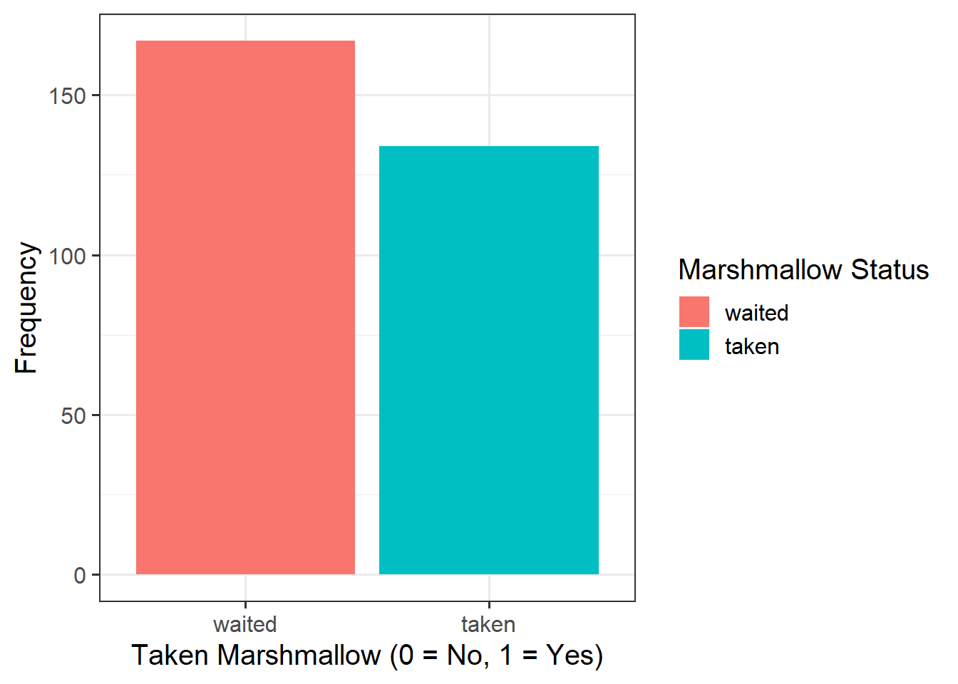
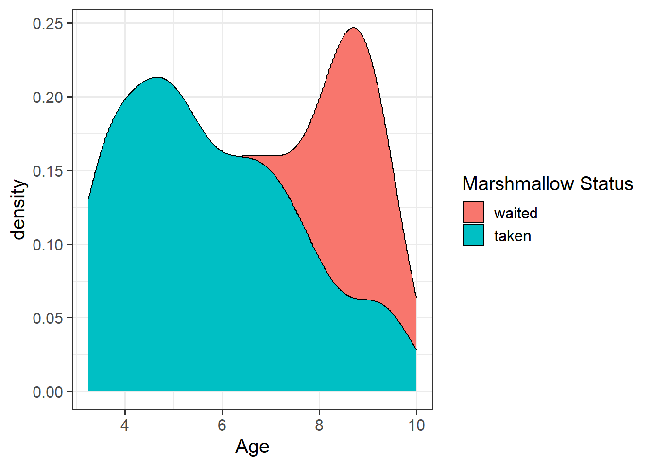
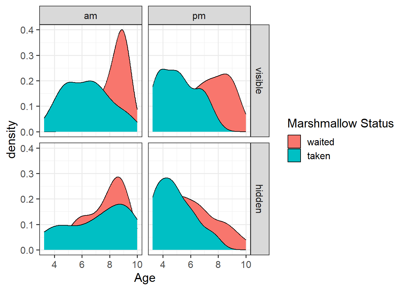
- For children aged 2 years old the log-odds of them taking the marshmallow are 3.76 + -0.62*2 = 2.52.
- Translating this to odds, we exponentiate it, so the odds of them taking the marshmallow are \(e^{(3.76 + -0.62*2)} = e^{2.52} = 12.43\).
(This is the same as \(e^{3.76} \times e^{-0.62*2}\))
- These odds of 12.43 means that (rounded to nearest whole number) if we take 13 children aged 2 years, we would expect 12 of them to take the marshmallow, and 1 to not take it.
- If we consider how the odds change for every extra year of age (i.e. for 3 year old as opposed to 2 year old children):
- the log-odds of taking the marshmallow decrease by -0.62.
- the odds of taking the marshmallow are multiplied by 0.54.
- so for a 3 year old child, the odds are \(12.43 \times 0.54 = 6.69\).
(And we can also calculate this as \(e^{2.52 + -0.62}\))
- So we have gone from odds of 12.4-to-1 for 2 year olds, and 6.7-to-1 for 3 year olds. The odds have been multiplied by 0.54.
But those odds, when converted to probability, these are 0.93 and 0.87. So \(0.54 \times odds\) is not \(0.54 \times probability\).
Because our intercept is at a single point (it’s not an association), we can actually convert this to a probability. Remember that \(odds = \frac{p}{1-p}\), which means that \(p = \frac{odds}{1 + odds}\). So the probability of taking the marshmallow for a child aged zero is \(\frac{43.13}{1 + 43.13} = 0.98\).
Unfortunately, we can’t do the same for any slope coefficients. This is because while the intercept is “odds”, the slopes are “odds ratios” (i.e. changes in odds), and changes in odds are different at different levels of probability.
Consider how when we multiply odds by 2, the increase in probability is not constant:
| 0.5 |
\(\frac{1}{1+0.5} = 0.33\) |
| 1 |
\(\frac{1}{1+1} = 0.5\) |
| 2 |
\(\frac{2}{1+2} = 0.66\) |
| 4 |
\(\frac{4}{1+4} = 0.8\) |
| 8 |
\(\frac{8}{1+8} = 0.88\) |
In R:
To translate log-odds to odds in order to aid interpretation, we can exponentiate (i.e., by using exp()) the coefficients from your model using R via the following command:
We can also use R to extract predicted probabilities for us from our models.
- Calculate the predicted log-odds (probabilities on the logit scale):
predict(model, type="link")
- Calculate the predicted probabilities:
predict(model, type="response")
Generalized Linear Models
Generalized linear models can be fitted in R using the glm function, which is similar to the lm function for fitting linear models. However, we also need to specify the family (i.e., link) function. There are three key components to consider:
- Random component / probability distribution - The distribution of the response/outcome variable. Can be from any family of distributions as listed below.
- Systematic component / linear predictor - the explanatory/predictor variable(s) (can be continuous or discrete).
- Link function - specifies the link between a random and systematic components.
Formula:
\(y_i = \beta_0 + \beta_1 x_i + + \beta_2 x_i + \epsilon_i\)
In R:
glm(y ~ x1 + x2, data = data, family = <INSERT_FAMILY>)
The family argument takes (the name of) a family function which specifies the link function and variance function (as well as a few other arguments not entirely relevant to the purpose of this course).
The exponential family functions available in R are:
-
binomial (link = “logit”)
-
gaussian (link = “identity”)
-
poisson (link = “log”)
-
Gamma (link = “inverse”)
-
inverse.gaussian (link = “1/mu2”)
See ?glm for other modeling options. See ?family for other allowable link functions for each family.
Drop-in-Deviance Test to Compare Mested Models
When moving from linear regression to more advanced and flexible models, testing of goodness of fit is more often done by comparing a model of interest to a simpler one.
The only caveat is that the two models need to be nested, i.e. one model needs to be a simplification of the other, and all predictors of one model needs to be within the other.
We want to compare the model we previously fitted against a model where all slopes are 0, i.e. a baseline model:
\[
\begin{aligned}
M_1 : \qquad\log \left( \frac{p}{1 - p} \right) &= \beta_0 \\
M_2 : \qquad \log \left( \frac{p}{1 - p} \right) &= \beta_0 + \beta_1 x
\end{aligned}
\]
In R: We do the comparison as follows:
mdl_reduced <- glm(DV ~ 1, family = "binomial", data = dataset)
mdl_main <- glm(DV ~ IV1 + IV2 ... + IV4, family = "binomial", data = dataset)

anova(mdl_red, mdl_main, test = 'Chisq')
In the output we can see the residual deviance of each model. Remember the deviance is the equivalent of residual sum of squares in linear regression.
Akaike and Bayesian Information Criteria
Deviance measures lack of fit, and it can be reduced to zero by making the model more and more complex, effectively estimating the value at each single data point. However, this involves adding more and more predictors, which makes the model more complex (and less interpretable).
Typically, the simpler model should be preferred when it can still explain the data almost as well. This is why information criteria were devised, exactly to account for both the model misfit but also its complexity.
\[
\text{Information Criterion} = \text{Deviance} + \text{Penalty for model complexity}
\]
Depending on the chosen penalty, you get different criteria. Two common ones are the Akaike and Bayesian Information Criteria, AIC and BIC respectively:
\[
\begin{aligned}
\text{AIC} &= \text{Deviance} + 2 p \\
\text{BIC} &= \text{Deviance} + p \log(n)
\end{aligned}
\]
where \(n\) is the sample size and \(p\) is the number of regression coefficients in the model. Models that produce smaller values of these fit criteria should be preferred.
AIC and BIC differ in their degrees of penalization for number of regression coefficients, with BIC usually favouring models with fewer terms.
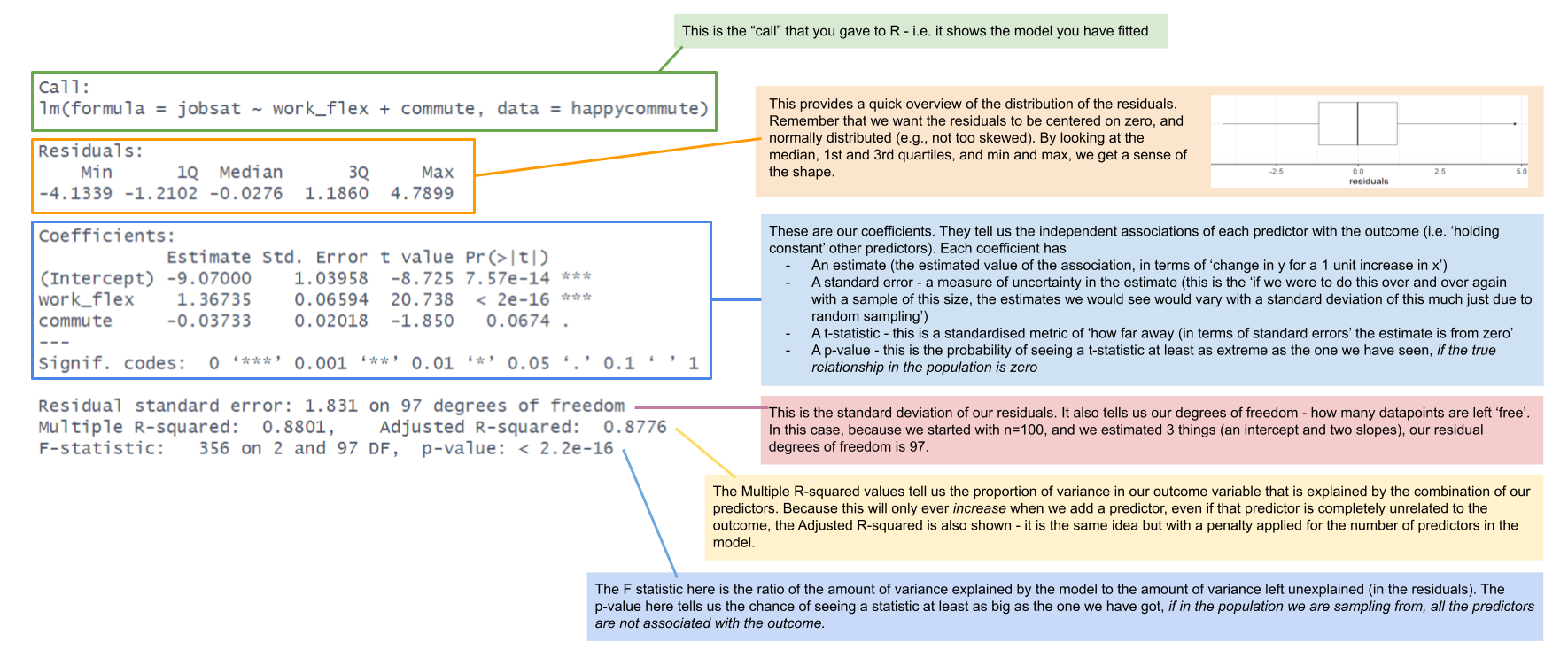
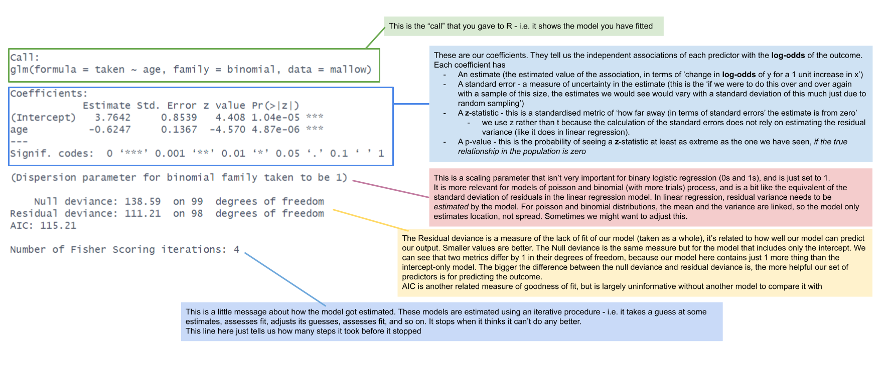
Comparing lm() and glm() summary output
