Errors, Power, Effect size, Assumptions

Semester 2 - Week 5

1 Formative Report C

1.1 Instructions and data

Instructions and data were released in week 1 of semester 2.

This week: Submission of Formative Report C

• Your group must submit one PDF file for formative report C by 12 noon on Friday 16th of February 2024.
  • No extensions are possible for group-based reports, see “Assessment Information” page on LEARN.
  • To submit, go to the course Learn page > click “Assessment” > click “Submit Formative Report C (PDF file only)”.
  • Only one person per group is required to submit on behalf of the entire group.
  • Ensure that everyone in the group has joined the group on LEARN. Otherwise, you won’t see the feedback.
• The submitted report must be a PDF file of max 6 sides of A4 paper.
  • Keep the default settings in terms of Rmd knitting font and page margins.
  • Ensure your report title includes the group name: Group NAME.LETTER
  • In the author section, ensure the report lists the exam numbers of all group members: B000001, B000002, …
• At the end of the file, you will place the appendices and these will not count towards the six-page limit.

  • You can include an optional appendix for additional tables and figures which you can’t fit in the main part of the report;

  • You must include a compulsory appendix listing all of the R code used in the report. This is done automatically if you end your file with the following section, which is already included in the template Rmd file:

    # Appendix: R code
    
    ```{r ref.label=knitr::all_labels(), echo=TRUE, eval=FALSE}
    
    ```

  • Excluding the Appendix, the report should not include any reference to R code or functions, but be written for a generic reader who is only assumed to have a basic statistical understanding without any R knowledge.

• In Flexible Learning Week (FLW, next week)
  • There will be no lectures
  • The labs are still on - please go to the labs to receive feedback on your submission
  • In the labs (a) check the formative feedback, and (b) study the example solutions and ask questions to tutors on code that is unclear.

1.2 This week’s task

Task C5

Compute and report the effect size, check if the assumptions underlying the t-test are violated.

Sub-steps

Below there are sub-steps you need to consider to complete this week’s task.

Tip

To see the hints, hover your cursor on the superscript numbers.

• Reopen last week’s Rmd file, as you will continue last week’s work and build on it.¹

• Compute an effect size for the graduation rate of female students.²

• Add a write-up of the effect size computed above to the report. After reporting whether the t-test results are statistically significant, also discuss whether your results also have practical significance (i.e. are important).

• Check and report whether the t-test assumptions are satisfied.³

• Add a write-up of the assumptions checks to your report.

• Knit the report to PDF and submit it via LEARN before the deadline (12 noon on the 16 February 2024).

2 Worked Example

The R code is visible for instructional purposes only, but it should not be visible in a PDF report. No R code or output should be visible in a report - only text, figures, and tables. Of course, Appendix B should have R code visible.

R code

library(tidyverse)
library(patchwork)
library(kableExtra)

pass_scores <- read_csv("https://uoepsy.github.io/data/pass_scores.csv")
dim(pass_scores)
head(pass_scores)
glimpse(pass_scores)

summary(pass_scores)

plt_hist <- ggplot(pass_scores, aes(x = PASS)) + 
    geom_histogram(color = 'white') +
    labs(x = "PASS scores", title = "(a) Histogram")

plt_box <- ggplot(pass_scores, aes(x = PASS)) + 
    geom_boxplot() +
    labs(x = "PASS scores", title = "(b) Boxplot")

plt_hist / plt_box

stats <- pass_scores %>%
    summarise(n = n(),
              Min = min(PASS),
              Max = max(PASS),
              M = mean(PASS),
              SD = sd(PASS))

kbl(stats, booktabs = TRUE, digits = 2, 
    caption = "Descriptive statistics for PASS scores")

# Confidence interval
xbar <- stats$M
s <- stats$SD
n <- stats$n
se <- s / sqrt(n)
tstar <- qt(c(0.025, 0.975), df = n - 1)

xbar + tstar * se

# observed t-statistic
tobs <- (xbar - 33) / se
tobs

# p-value method
pvalue <- 2 * pt(abs(tobs), df = n - 1, lower.tail = FALSE)
pvalue

# critical values method
tstar
tobs

# effect size
D <- (xbar - 33) / s
D

# assumptions checks
dim(pass_scores)

plt_dens <- ggplot(pass_scores, aes(x = PASS)) + 
    geom_density() +
    labs(x = "PASS scores",
         title = "(a) Density plot")

plt_qq <- ggplot(pass_scores, aes(sample = PASS)) + 
    geom_qq() +
    geom_qq_line() +
    labs(x = "Theoretical quantiles",
         y = "Sample quantiles",
         title = "(b) QQ-plot")

plt_dens | plt_qq

shapiro.test(pass_scores$PASS)

Introduction

A random sample of 20 students from the University of Edinburgh completed a questionnaire measuring their total endorsement of procrastination. The data, available from https://uoepsy.github.io/data/pass_scores.csv, were used to estimate the average procrastination score of all Edinburgh University students, as well as testing whether the mean procrastination score differed from the Solomon & Rothblum reported average of 33 at the 5% significance level. The recorded variables include a subject identifier (sid, categorical), the school each belongs to (school, categorical), and the total score on the Procrastination Assessment Scale for Students (PASS, numeric). The data did not include any impossible values for the PASS scores, as they were all within the possible range of 0 – 90. To answer the questions of interest, we only focused on the total PASS score variable.

Analysis

Throughout the report we used a significance level \(\alpha\) of 5%.

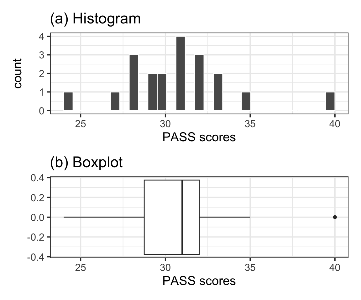
The distribution of PASS scores, as shown in Figure 1(a), is roughly bell shaped and does not have any impossible values. The outlier (40) depicted in the boxplot shown in Figure 1(b) is well within the range of plausible values for the PASS scale (0–90) and as such was not removed for the analysis.

Figure 1: Distribution of PASS scores for a sample of Edinburgh University students

Table 1: Descriptive statistics for PASS scores

n	Min	Max	M	SD
20	24	40	30.7	3.31

Table 1 displays summary statistics for the PASS scores in the sample of Edinburgh University students. From the sample data we obtain an average procrastination score of \(M = 30.7\), 95% CI [29.15, 32.25]. Hence, we are 95% confident that a Edinburgh University student will have a procrastination score between 29.15 and 32.25, which is between 0.75 and 3.85 lower than the average score of 33 reported by Solomon & Rothblum.

To investigate whether the mean PASS scores of all Edinburgh University students, \(\mu\) say, differs from the Solomon & Rothblum reported average of 33, we performed a one sample t-test of \(H_0 : \mu = 33\) against \(H_1 : \mu \neq 33\). The sample data provided very strong evidence against the null hypothesis and in favour of the alternative one that the mean procrastination score of Edinburgh University students is significantly different from the Solomon & Rothblum reported average of 33: \(t(19) = -3.11, p = .006\), two-sided. The size of the effect was also found to be medium to large \((D = -0.69)\).

Figure 2: Density plot (a) and QQ-plot (b) of PASS scores for a sample of Edinburgh University students

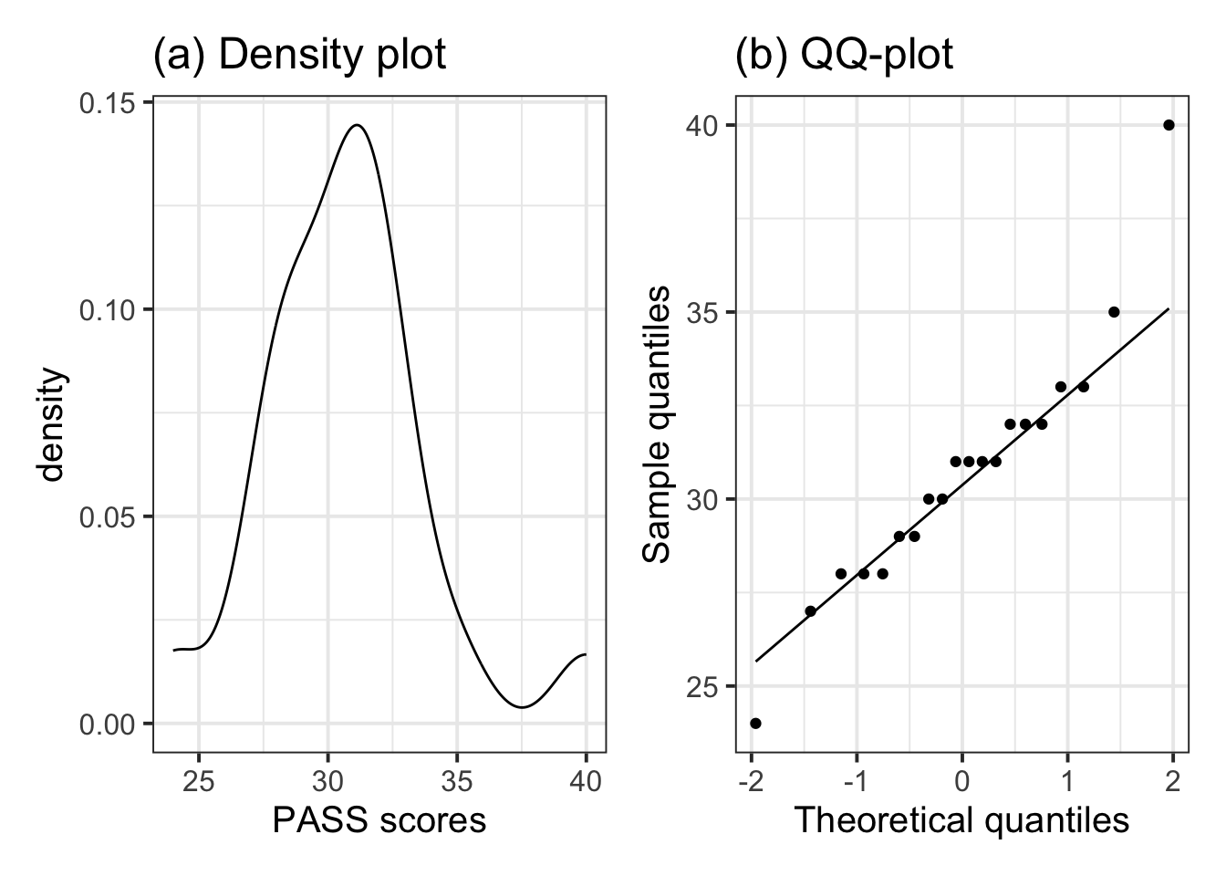
The sample data did not show violations of the assumptions required for the t-test results to be valid. Specifically, the data were collected on a random sample of students from Edinburgh University, hence independence was met. Figure 2(a) shows that the distribution of PASS scores is roughly bell-shaped, with a single mode and as such does not raise any concerns of violations of normality. Similarly, the QQ-plot in Figure 2(b) shows agreement between the sample and theoretical quantiles, as they almost all fall on the line. We also performed a Shapiro-Wilk test against the null hypothesis of normality of the population data: \(W = 0.94\), \(p = .20\). The sample data did not provide sufficient evidence at the 5% level to reject the null hypothesis that the population data follow a normal distribution.

Discussion

Data including the Procrastination Assessment Scale for Students (PASS) scores for a random sample of 20 students at Edinburgh University were used to estimate the average procrastination score for a student of that university. In addition, the data were used to test whether there is a significant difference between that average score and the Solomon & Rothblum reported average of 33.

The data provided very strong evidence that the mean procrastination score of Edinburgh University students differs from 33. Furthermore, the data indicate that a Edinburgh University student tends to have a mean procrastination score between 29.15 and 32.35, which is 0.75 and 3.85 lower than the Solomon & Rothblum reported average of 33.

What is missing from this instructional example:

• Appendix A
• Appendix B

Footnotes

1. Hint: Ask last week’s driver for the Rmd file, they should share it with the group via email or the group discussion space. To download the file from the server, go to the RStudio Files pane, tick the box next to the Rmd file, and select More > Export.

2. Hint: Cohen’s \(D\) for a one sample t-test is given by

   \[D = \frac{\bar{x} - \mu_0}{s}\]

   where \(\bar{x}\) is the sample mean, \(\mu_0\) is the value for the population mean that we hypothesised in the null hypothesis (50), and \(s\) is the sample standard deviation.

3. Hint: Recall that, for the t-test results to be valid, conditions (1) and (2) below need to be met:

   1. The data need to come from a random sample of the population
   2. Either one of these holds:
      • The population follows a normal distribution
      • The sample size is large enough, \(n \geq 30\) as a guideline.

   For (1), this is known from the study design description. For (2) some of these functions may be useful: dim, nrow, geom_qq, geom_qq_line, shapiro.test.