Your group must submit one PDF file for formative report C by 12 noon on Friday the 16th of February 2024 (next week).
To submit go to the course Learn page, click “Assessment”, then click “Submit Formative Report C (PDF file only)”.
No extensions. As mentioned in the Assessment Information page, no extensions are possible for group-based reports.
1.2 This week’s task
Task C4
Tidy up your report so far, making sure to have 3 sections: introduction, analysis and discussion. After those, you can have Appendix A (additional figures or tables) and Appendix B (the R code used).
Sub-steps
Below there are sub-steps you need to consider to complete this week’s task.
Tip
To see the hints, hover your cursor on the superscript numbers.
Reopen last week’s Rmd file, as you will continue last week’s work and build on it.1
Ensure that your report has 3 sections:
Introduction - where you provide a brief description of the data, variables and their type, and the research questions you are going to address.
Analysis - where you show and describe your results. Please note that no R code or output should be visible, but only figures and tables.
Discussion - where you summarise your key results in a few take-home messages that answer the research questions.
Use the Some Helpful Formatting Resources section from week 1 of semester 2 to see (1) a checklist for successful knitting, (2) APA style guidelines, (3) how to hide code and/or output, and (4) how to change figure height and width.
Structure your Rmd file as follows:
---
title: "Formative report C (Group 0.A)"
author: "B000000, B000001, B00002, B00003, B000004"
date: "Write the date here"
output: bookdown::pdf_document2
toc: false
---
This is the metadata block. It includes the:
document title
author name
date (to leave empty, use an empty string "")
the output type
The output type could be html_document, pdf_document, etc.
We use bookdown::pdf_document2 so that we can reference figures, which pdf_document doesn’t let you do.
The code bookdown::pdf_document2 simply means to use the pdf_document2 type from the bookdown package.
The code toc: false hides the table of contents.
This code chunks contains your rough work from each week. Give names to plots and tables, so that you can reference those later on. The option include=FALSE hides both code and output.
To run each line of code while you are working, put your cursor on the line and press Control + Enter on Windows or Command + Enter on a macOS.
## IntroductionWrite here an introduction to the data, the variables, and anything worth of notice in the data.## AnalysisPresent here your tables, plots, and results. In the code chunk below, you do not need to put the chunk option `echo=FALSE` as you set this option globally in the setup chunk. ```{r}pltEye```If you didn't set it globally, you would need to put it in the chunk options:```{r, echo=FALSE}pltEye```More text...## DiscussionWrite up your take home messages here...
This contains your actual textual reporting, as well as tables and figures. To show in place a plot previously created, just include the plot name in a code chunk with the option echo = FALSE to hide the code but display the output.
## Appendix A - Additional tables and figures

Insert here any additional tables or figures that you could not fit in the
page limit.
## Appendix B - R code```{r ref.label=knitr::all_labels(), echo=TRUE, eval=FALSE}```
Copy and paste in your report this last code chunk as it is here. This special code chunk will copy here all the previous R code chunks that you have created and automatically populate Appendix B for you.
Note: The appendices do not count towards the 6-page limit.
2 Worked Example
The R code is visible here for instructional purposes only, but it should not be visible in a PDF report. It should only appear as part of the appendix.
stats<-pass_scores%>%summarise(n =n(), Min =min(PASS), Max =max(PASS), M =mean(PASS), SD =sd(PASS))kbl(stats, booktabs =TRUE, digits =2, caption ="Descriptive statistics for PASS scores")# Confidence intervalxbar<-stats$Ms<-stats$SDn<-stats$nse<-s/sqrt(n)tstar<-qt(c(0.025, 0.975), df =n-1)xbar+tstar*se# observed t-statistictobs<-(xbar-33)/setobs# p-value methodpvalue<-2*pt(abs(tobs), df =n-1, lower.tail =FALSE)pvalue# critical value methodtstartobs
Introduction
A random sample of 20 students from the University of Edinburgh completed a questionnaire measuring their total endorsement of procrastination. The data, available from https://uoepsy.github.io/data/pass_scores.csv, were used to estimate the average procrastination score of all Edinburgh University students, as well as testing whether the mean procrastination score differed from the Solomon & Rothblum reported average of 33 at the 5% significance level. The recorded variables include a subject identifier (sid, categorical), the school each belongs to (school, categorical), and the total score on the Procrastination Assessment Scale for Students (PASS, numeric). The data do not include any impossible values for the PASS scores, as they were all within the possible range of 0 – 90. To answer the questions of interest, in the following we will only focus on the total PASS score variable.
Analysis
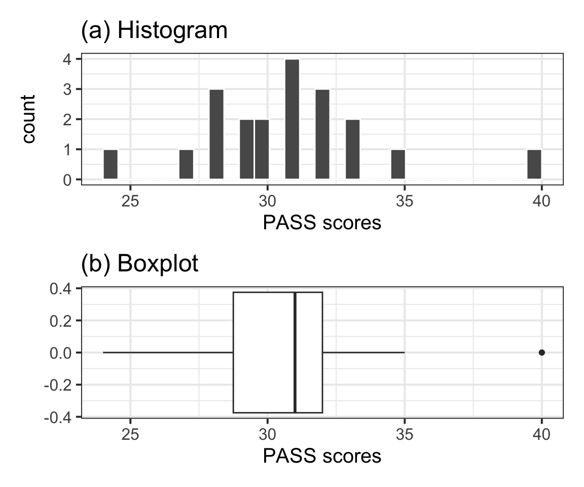
The distribution of PASS scores, as shown in Figure 1(a), is roughly bell shaped and does not have any impossible values. The outlier (40) depicted in the boxplot shown in Figure 1(b) is well within the range of plausible values for the PASS scale (0–90) and as such was not removed for the analysis.
Figure 1: Distribution of PASS scores for a sample of Edinburgh University students
Table 1: Descriptive statistics for PASS scores
n
Min
Max
M
SD
20
24
40
30.7
3.31
Table 1 displays summary statistics for the PASS scores in the sample of Edinburgh University students. From the sample data we obtain an average procrastination score of \(M = 30.7\), 95% CI [29.15, 32.25]. Hence, we are 95% confident that a Edinburgh University student will have a procrastination score between 29.15 and 32.25, which is between 0.75 and 3.85 lower than the average score of 33 reported by Solomon & Rothblum.
Let \(\mu\) denote the mean PASS score of all Edinburgh University students. At the 5% significance level, we performed a one sample t-test of \(H_0 : \mu = 33\) against \(H_1 : \mu \neq 33\). The sample data provide very strong evidence against the null hypothesis and in favour of the alternative one that the mean procrastination score of Edinburgh University students is significantly different from the Solomon & Rothblum reported average of 33: \(t(19) = -3.11, p = .006\), two-sided.
Discussion
Data including the Procrastination Assessment Scale for Students (PASS) scores for a random sample of 20 students at Edinburgh University we used to estimate the average procrastination score for a student of that university. In addition, the data were used to test whether there is a significant difference between that average score and the Solomon & Rothblum reported average of 33.
We are 95% confident that a Edinburgh University student will have a procrastination score between 29.15 and 32.25. Furthermore, at the 5% significance level, the data provide very strong evidence that the mean procrastination score of Edinburgh University students is different from 33. The confidence interval, reported above, indicates that a Edinburgh University student tends to have a mean procrastination score between 0.75 and 3.85 lower than the Solomon & Rothblum reported average of 33.
Hint: Ask last week’s driver for the Rmd file, they should share it with the group via email or the group discussion space. To download the file from the server, go to the RStudio Files pane, tick the box next to the Rmd file, and select More > Export.↩︎