| Variable Name | Description |
|---|---|
| sid | Subject identifier |
| school | School each subject belonged to |
| PASS | Total endorsement of procrastination score |
Hypothesis testing: p-values
Semester 2 - Week 2
1 Formative Report C
1.1 Instructions and data
Instructions and data were released in week 1 of semester 2.
1.2 This week’s task
Task C2
At the 5% significance level and using the p-value method, test whether the 2012 mean graduation rate for female students at colleges and universities in the United States is significantly different from a rate of 50 percent.
Sub-steps
Below there are sub-steps you need to consider to complete this week’s task.
Tip
To see the hints, hover your cursor on the superscript numbers.
- Reopen last week’s Rmd file, as you will continue last week’s work and build on it.1
- Specify the null and alternative hypotheses.2
- Compute the observed value of the t-statistic.3
The t-statistic follows a t-distribution with how many degrees of freedom? You will need this number for the next task.4
Compute the p-value for the test.5
Using a 5% significance level, i.e. \(\alpha = .05\), make a decision on whether or not to reject the null hypothesis.6
Provide a write up of your results in the context of the research question.
Update the report introduction to also include information about the second question being investigated, i.e. whether the mean graduation rate for female students at colleges and universities in the United States is significantly different from a rate of 50 percent.
2 Worked Example
The Procrastination Assessment Scale for Students (PASS) was designed to assess how individuals approach decision situations, specifically the tendency of individuals to postpone decisions (Solomon & Rothblum, 1984).
The PASS assesses the prevalence of procrastination in six areas: writing a paper; studying for an exam; keeping up with reading; administrative tasks; attending meetings; and performing general tasks. For a measure of total endorsement of procrastination, responses to 18 questions (each measured on a 1-5 scale) are summed together, providing a single score for each participant (range 0 to 90). The mean score from Solomon & Rothblum, 1984 was 33.
Research question:
Does the mean procrastination score of Edinburgh University students differ from the Solomon & Rothblum average of 33?
To answer this question, we will use data collected for a random sample of students from the University of Edinburgh: https://uoepsy.github.io/data/pass_scores.csv
Necessary packages:
- tidyverse for using
read_csv(), usingsummarise()andggplot(). - patchwork for arranging plots side by side or underneath
- kableExtra for creating user-friendly tables
Read the data into R:
To inspect the data:
head(pass_scores)# A tibble: 6 × 3
sid school PASS
<chr> <chr> <dbl>
1 s_1 GeoSciences 31
2 s_2 ECA 24
3 s_3 LAW 32
4 s_4 ECA 40
5 s_5 LAW 28
6 s_6 SSPS 31glimpse(pass_scores)Rows: 20
Columns: 3
$ sid <chr> "s_1", "s_2", "s_3", "s_4", "s_5", "s_6", "s_7", "s_8", "s_9", …
$ school <chr> "GeoSciences", "ECA", "LAW", "ECA", "LAW", "SSPS", "PPLS", "SLL…
$ PASS <dbl> 31, 24, 32, 40, 28, 31, 30, 28, 32, 29, 28, 33, 35, 33, 30, 31,…summary(pass_scores) sid school PASS
Length:20 Length:20 Min. :24.00
Class :character Class :character 1st Qu.:28.75
Mode :character Mode :character Median :31.00
Mean :30.70
3rd Qu.:32.00
Max. :40.00 Visualise the distribution of PASS scores:
Note
The boxplot highlights an outlier (40). However, this value is well within the plausible range of the scale (0 – 90), hence it is of no concern and the point can be kept for the analysis.
plt_hist <- ggplot(pass_scores, aes(x = PASS)) +
    geom_histogram(color = 'white')

plt_box <- ggplot(pass_scores, aes(x = PASS)) +
    geom_boxplot()

plt_hist / plt_box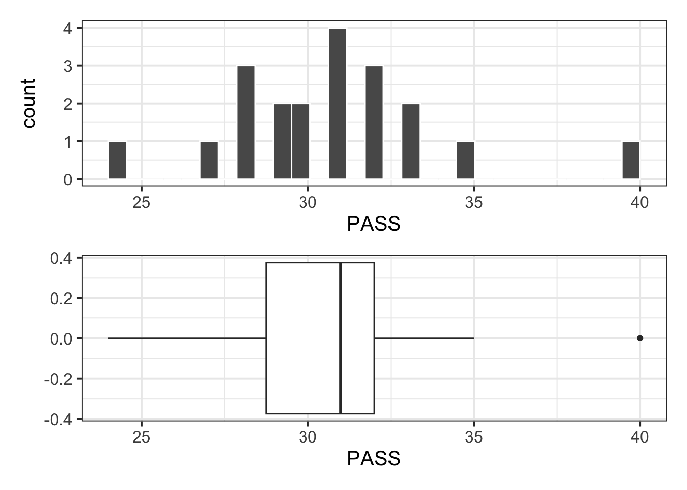
Descriptive statistics:
| n | Min | Max | M | SD |
|---|---|---|---|---|
| 20 | 24 | 40 | 30.7 | 3.31 |
Step 1: Identify the null and alternative hypotheses.
First we need to write the null and alternative hypothesis, which take the form \(H_0 : \mu = \mu_0\) vs \(H_1: \mu \neq \mu_0\). From the research question, we identify the hypothesised value \(\mu_0\) to be 33, hence:
These are written as:
$$H_{0}: \mu = 33$$
$$H_{1}: \mu \neq 33$$
In H_{0} and H_{1} the 0 and 1 within curly braces are written as subscripts. The curly braces delimit what goes in the subscript. The symbol \mu denotes the greek letter “mu” that stands for the population mean (a parameter). The symbol \neq means not equal.
\[H_0: \mu = 33\] \[H_1: \mu \neq 33\]
Step 2: Compute the t-statistic
Next, we compute the t-statistics, which compares the difference between the sample and hypothesised mean (\(\bar{x} - \mu_0\)) to the variation due to random sampling (\(SE_{\bar{x}}\)).
To test the hypothesis, we need to compute the t-statistic,
\[ t = \frac{\bar{x} - \mu_0}{SE_{\bar{x}}} \qquad \text{where} \qquad SE_{\bar{x}} = \frac{s}{\sqrt{n}} \]
# Sample mean
xbar <- stats$M

# Standard error
s <- stats$SD
n <- stats$n
se <- s / sqrt(n)

# Observed t-statistic
tobs <- (xbar - 33) / se
tobs
[1] -3.107272Step 3: Identify the null distribution, i.e. the distribution of the t-statistic assuming the null to be true.
As the sample size is \(n =\) 20, if the null hypothesis is true the t-statistic will follow a t(19) distribution.
Step 4: Compute the p-value
As the alternative hypothesis is two-sided (or two-tailed), we can compute the p-value as twice the area to the right of abs(tobs).
Step 5: Make a decision
Using the p-value method, we compare the p-value with the significance level (\(\alpha = .05\) in this case). As .005800318 < .05, we reject \(H_0\). Please note this is just an explanation and not how you would write up the result!
We can update the example introduction to add the new question investigated:
Example introduction
A random sample of 20 students from the University of Edinburgh completed a questionnaire measuring their total endorsement of procrastination. The data, available from https://uoepsy.github.io/data/pass_scores.csv, were used to estimate the average procrastination score of all Edinburgh University students, and whether the mean procrastination score differed from the Solomon & Rothblum reported average of 33 at the 5% significance level. The recorded variables included a subject identifier (sid), the school of each subject (school), and the total score on the Procrastination Assessment Scale for Students (PASS). The data do not include any impossible values for the PASS scores, as they were all within the possible range of 0 – 90. To answer the question of interest, in the following we will only focus on the total PASS score variable.
And this is a potential way to report the t-test results:
Example hypothesis test write-up
At the 5% significance level, the sample data provide very strong evidence against the null hypothesis and in favour of the alternative one that the mean procrastination score of Edinburgh University students is different from the Solomon & Rothblum reported average of 33: \(t(19) = -3.11, p = .006\), two-sided.
3 Student Glossary
To conclude the lab, add the new functions to the glossary of R functions.
| Function | (package) and use |
|---|---|
geom_histogram |
(tidyverse) creates a histogram |
geom_boxplot |
(tidyverse) creates a boxplot |
summarise |
(tidyverse) used to compute some summaries of data |
n() |
(tidyverse) when used inside of summarise(), it counts the number of rows |
mean |
compute the mean, i.e. the average |
sd |
compute the standard deviation, i.e. the square root of the variance |
abs |
absolute value, i.e. drop the sign |
pt |
compute the probability in a t-distribution to the left (by default) |
Footnotes
Hint: Ask last week’s driver for the Rmd file, they should share it with the group via email or the group discussion space. To download the file from the server, go to the RStudio Files pane, tick the box next to the Rmd file, and select More > Export.↩︎
-
Hint: Identify the hypothesised value of the mean, \(\mu_0\), and replace that value in the following equations:
\[H_{0} : \mu = \mu_{0}\] \[H_{1} : \mu \neq \mu_{0}\]
Code used to write the above:
$$ H_{0} : \mu = \mu_{0} $$
$$ H_{1} : \mu \neq \mu_{0} $$
We write mathematical equations in the text part of an Rmd file, i.e. not inside a code chunk. Wrap a mathematical equation with dollar signs to tell R when an equation starts and ends. Text written within curly braces after an underscore is rendered as a subscript, so
_{0}creates a subscript 0.↩︎ -
Hint: Use the following formula for the t-statistic:
\[t = \frac{\bar{x} - \mu_0}{SE_{\bar{x}}} \qquad \text{where} \qquad SE_{\bar{x}} = \frac{s}{\sqrt{n}}\]
In the above:
- \(\bar{x}\) is the sample mean
- \(\mu_0\) is the hypothesised value for the population mean
- \(s\) is the sample standard deviation
- \(n\) is the sample size
Hint: the t-statistic follows a \(t(n-1)\) distribution where \(n-1\) are the degrees of freedom. In the next task, you will need to provide the degrees of freedom to the
pt()function.↩︎Hint: compare the p-value with the significance level.
If p-value \(\leq \alpha\), reject. Otherwise, do not reject.↩︎