Path Analysis
Packages for today
- lavaan
- semPlot or tidySEM
Introducing Path Analysis
over last couple of weeks we have applied exploratory and then confirmatory factor analysis to develop and then test factor analysis models of ‘conduct problems.’ Factor models posit the existence of some underlying latent variable which is thought of as resulting in the scores on our measured items. Especially in Week 8 we began to depict the variables and parameters involved in these models visually, in what get called ‘path’ or ‘SEM’ diagrams. Specifically, by using rectangles (observed variables), ovals (latent variables), single headed arrows (regression paths) and double headed arrows (covariances), we could draw various model structures.
This week, we are temporarily putting aside the latent variables (no ovals in the drawings today!) and focusing on some of the fundamentals that motivate this modeling approach.
Mountains cannot be surmounted except by winding paths
Over the course of USMR and the first block of this course, you have hopefully become pretty comfortable with the regression world, and can see how it is extended to lots of different types of outcome and data stuctures.
If we are for the time being ignoring the latent variables, then what exactly do we gain by this approach of drawing out our variables and drawing various lines between them? Surely our regression toolkit can do all the things we need?
Let’s imagine we are interested in peoples’ intention to get vaccinated, and we observe the following variables:
- Intention to vaccinate (scored on a range of 0-100)
- Health Locus of Control (HLC) score (average score on a set of items relating to perceived control over ones own health)
- Religiosity (average score on a set of items relating to an individual’s religiosity).
We are assuming here that we do not have the individual items, but only the scale scores (if we had the individual items we might be inclined to model religiosity and HLC as latent variables!).
If we draw out our variables, and think about this in the form of a standard regression model with “Intention to vaccinate” as our outcome variable, then all the lines are filled in for us (see Figure 1)

Figure 1: Multiple regression as a path model
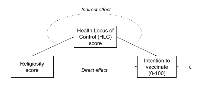
But what if our theory suggests that some other model might be of more relevance? For instance, what if we believe that participants’ religiosity has an effect on their Health Locus of Control score, which in turn affects the intention to vaccinate (see Figure 2)?
In this case, the HLC variable is thought of as a mediator, because is mediates the effect of religiosity on intention to vaccinate. We are specifying presence of a distinct type of effect: direct and indirect.
Direct vs Indirect
In path diagrams:
- Direct effect = one single-headed arrow between the two variables concerned
- Indirect effect = An effect transmitted via some other variables

Figure 2: Mediation as a path model
The only option here is to conduct several regression models, because we have multiple endogenous variables. Fortunately, path analysis allows us to do just that - fit simultaneous regression equations!
Terminology refresher
- Exogenous variables are a bit like what we have been describing with words like “independent variable” or “predictor.” In a path diagram, they have no paths coming from other variables in the system, but have paths going to other variables.
- Endogenous variables are more like the “outcome”/“dependent”/“response” variables we are used to. They have some path coming from another variable in the system (and may also - but not necessarily - have paths going out from them).
Recall our way of drawing path diagrams (excluding any mention of latent variables and factors for now):
- Observed variables are represented by squares or rectangles. These are the named variables of interest which exist in our dataset - i.e. the ones which we have measured directly.
- Covariances are represented by double-headed arrows. In many diagrams these are curved.
- Regressions are shown by single headed arrows (e.g., an arrow from \(x\) to \(y\) for the path \(y~x\)).
Some key assumptions
There are a few assumptions of a complete path diagram:
- all our exogenous variables are correlated (unless we specifically assume that their correlation is zero)
- All models are ‘recursive’ (no two-way causal relations, no feedback loops)
- Residuals are uncorrelated with exogenous variables
- Endogenous variables are not connected by correlations (we would use correlations between residuals here, because the residuals are not endogenous)
- All ‘causal’ relations are linear and additive
- ‘causes’ are unitary (if A -> B and A -> C, then it is presumed that this is the same aspect of A resulting in a change in both B and C, and not two distinct aspects of A, which would be better represented by two correlated variables A1 and A2).
Causal??
It is a slippery slope to start using the word ‘cause,’ and personally I am not that comfortable using it here. However, you will likely hear it a lot in resources about path analysis and SEM, so it is best to be warned.
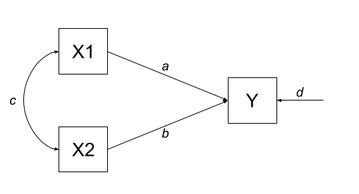
Please keep in mind that we are using a very broad definition of ‘causal,’ simply to reflect the one way nature of the relationship we are modeling. In Figure 3, a change in the variable X1 is associated with a change in Y, but not vice versa.

Figure 3: Paths are still just regressions.
Tracing rules
Thanks to Sewal Wright, we can express the correlation between any two variables in the system as the sum of all compound paths between the two variables.
compound paths are any paths you can trace between A and B for which there are:
- no loops
- no going forward then backward
- maximum of one curved arrow per path
Let’s consider the example below, for which the paths are all labelled with lower case letters \(a, b, c, \text{and } d\).

Figure 4: A multiple regression model as a path diagram
According to Wright’s tracing rules above, write out the equations corresponding to the 3 correlations between our observed variables (remember that \(r_{a,b} = r_{b,a}\), so it doesn’t matter at which variable we start the paths).
- \(r_{x1,x2} = c\)
- \(r_{x1,y} = a + bc\)
- \(r_{x2,y} = b + ac\)
Now let’s suppose we observed the following correlation matrix:
egdat <- read_csv("https://uoepsy.github.io/data/patheg.csv")
round(cor(egdat),2)
## x1 x2 y
## x1 1.00 0.36 0.75
## x2 0.36 1.00 0.60
## y 0.75 0.60 1.00We can plug these into our system of equations:
- \(r_{x1,x2} = c = 0.36\)
- \(r_{x1,y} = a + bc = 0.75\)
- \(r_{x2,y} = b + ac = 0.60\)
And with some substituting and rearranging, we can work out the values of \(a\), \(b\) and \(c\).
We can even work out what the path labeled \(d\) (the residual variance) is. First we sum up all the equations for the paths from Y to Y. These are:
- \(a^2\) (from Y to X1 and back)
- \(b^2\) (from Y to X2 and back)
- \(acb\) (from Y to X1 to X2 to Y)
- \(bca\) (from Y to X2 to X1 to Y)
Summing them all up and solving gives us:
\[
\begin{align}
r_{y \cdot x1, x2} & = a^2 + b^2 + acb + bca\\
& = 0.61^2 + 0.38^2 + 2 \times(0.61 \times 0.38 \times 0.36)\\
& = 0.68 \\
\end{align}
\]
We can think of this as the portion of the correlation of Y with itself that occurs via the predictors. Put another way, this is the amount of variance in Y explained jointly by X1 and X2, which sounds an awful lot like an \(R^2\)!
This means that the path \(d = \sqrt{1-R^2}\).
Hooray! We’ve just worked out regression coefficients when all we had was the correlation matrix of the variables! It’s important to note that we have been using the correlation matrix, so, somewhat unsurprisingly, our estimates are standardised coefficients.
Because we have the data itself, let’s quickly find them with lm()
# quickly scale all the columns in the data
egdat <- egdat %>% mutate_all(~scale(.)[,1])
# extract the coefs
coef(lm(y~x1+x2, egdat))
## (Intercept) x1 x2
## 1.943428e-16 6.118072e-01 3.816321e-01# extract the r^2
summary(lm(y~x1+x2, egdat))$r.squared## [1] 0.6884071Path Mediation
Now that we’ve seen how path analysis works, we can use that same logic to investigate models which have quite different structures, such as those including mediating variables. So if we can’t fit our theoretical model into a regression framework, let’s just fit it into a framework which is lots of regressions smushed together!Luckily, we can just get the lavaan package to do all of this for us. So let’s look at fitting the model below.
. I haven't properly read it though!](images/path/path2.png)
Figure 5: If you’re interested, you can find the inspiration for this data from the paper here. I haven’t properly read it though!
First we read in our data:
vax <- read_csv("https://uoepsy.github.io/data/vaxdat.csv")
summary(vax)
## religiosity hlc intention
## Min. :-1.000 Min. :0.400 Min. :39.00
## 1st Qu.: 1.800 1st Qu.:2.000 1st Qu.:59.00
## Median : 2.400 Median :3.000 Median :64.00
## Mean : 2.396 Mean :2.992 Mean :65.09
## 3rd Qu.: 3.000 3rd Qu.:3.600 3rd Qu.:74.00
## Max. : 4.600 Max. :5.800 Max. :88.00Then we specify the relevant paths:
med_model <- "
    intention ~ religiosity
    intention ~ hlc
    hlc ~ religiosity
"
If we fit this model as it is, we won’t actually be testing the indirect effect, we will simply be fitting a couple of regressions.
To do that, we need to explicitly define the indirect effect in the model, by first creating a label for each of its sub-component paths, and then defining the indirect effect itself as the product (why the product? Click here for a lovely pdf explainer from Aja).
To do this, we use a new operator, :=.
med_model <- "
    intention ~ religiosity
    intention ~ a*hlc
    hlc ~ b*religiosity

    indirect:=a*b
"
:=
This operator ‘defines’ new parameters which take on values that are an arbitrary function of the original model parameters. The function, however, must be specified in terms of the parameter labels that are explicitly mentioned in the model syntax.
Note. The labels we use are completely up to us. This would be equivalent:
med_model <- "
    intention ~ religiosity
    intention ~ peppapig * hlc
    hlc ~ kermit * religiosity

    indirect:= kermit * peppapig
"
Estimating the model
It is common to estimate the indirect effect using bootstrapping (a method of resampling the data with replacement, thousands of times, in order to empirically generate a sampling distribution). We can do this easily in lavaan:
mm1.est <- sem(med_model, data=vax, se = "bootstrap")
summary(mm1.est, ci = TRUE)
## lavaan 0.6-8 ended normally after 26 iterations
##
## Estimator ML
## Optimization method NLMINB
## Number of model parameters 5
##
## Number of observations 100
##
## Model Test User Model:
##
## Test statistic 0.000
## Degrees of freedom 0
##
## Parameter Estimates:
##
## Standard errors Bootstrap
## Number of requested bootstrap draws 1000
## Number of successful bootstrap draws 1000
##
## Regressions:
## Estimate Std.Err z-value P(>|z|) ci.lower ci.upper
## intention ~
## religiosty 0.270 1.041 0.260 0.795 -1.700 2.470
## hlc (a) 5.971 0.944 6.325 0.000 4.037 7.768
## hlc ~
## religiosty (b) 0.508 0.087 5.853 0.000 0.337 0.686
##
## Variances:
## Estimate Std.Err z-value P(>|z|) ci.lower ci.upper
## .intention 62.090 7.837 7.923 0.000 45.128 75.825
## .hlc 0.753 0.108 7.009 0.000 0.539 0.951
##
## Defined Parameters:
## Estimate Std.Err z-value P(>|z|) ci.lower ci.upper
## indirect 3.033 0.678 4.475 0.000 1.844 4.463Exercises
This week’s lab focuses on the technique of path analysis using the same context as previous weeks: conduct problems in adolescence. In this week’s example, a researcher has collected data on n=557 adolescents and would like to know whether there are associations between conduct problems (both aggressive and non-aggressive) and academic performance and whether the relations are mediated by the quality of relationships with teachers.
First, read in the dataset from https://uoepsy.github.io/data/cp_teachacad.csv
Use the sem() function in lavaan to specify and estimate a straightforward linear regression model to test whether aggressive and non-aggressive conduct problems significantly predict academic performance.
How do your results compare to those you obtain using the lm() function?
Now specify a model in which non-aggressive conduct problems have both a direct and indirect effect (via teacher relationships) on academic performance
Now define the indirect effect in order to test the hypothesis that non-aggressive conduct problems have both a direct and an indirect effect (via teacher relationships) on academic performance.
Fit the model and examine the 95% CI.
Specify a new parameter which is the total (direct+indirect) effect of non-aggressive conduct problems on academic performance
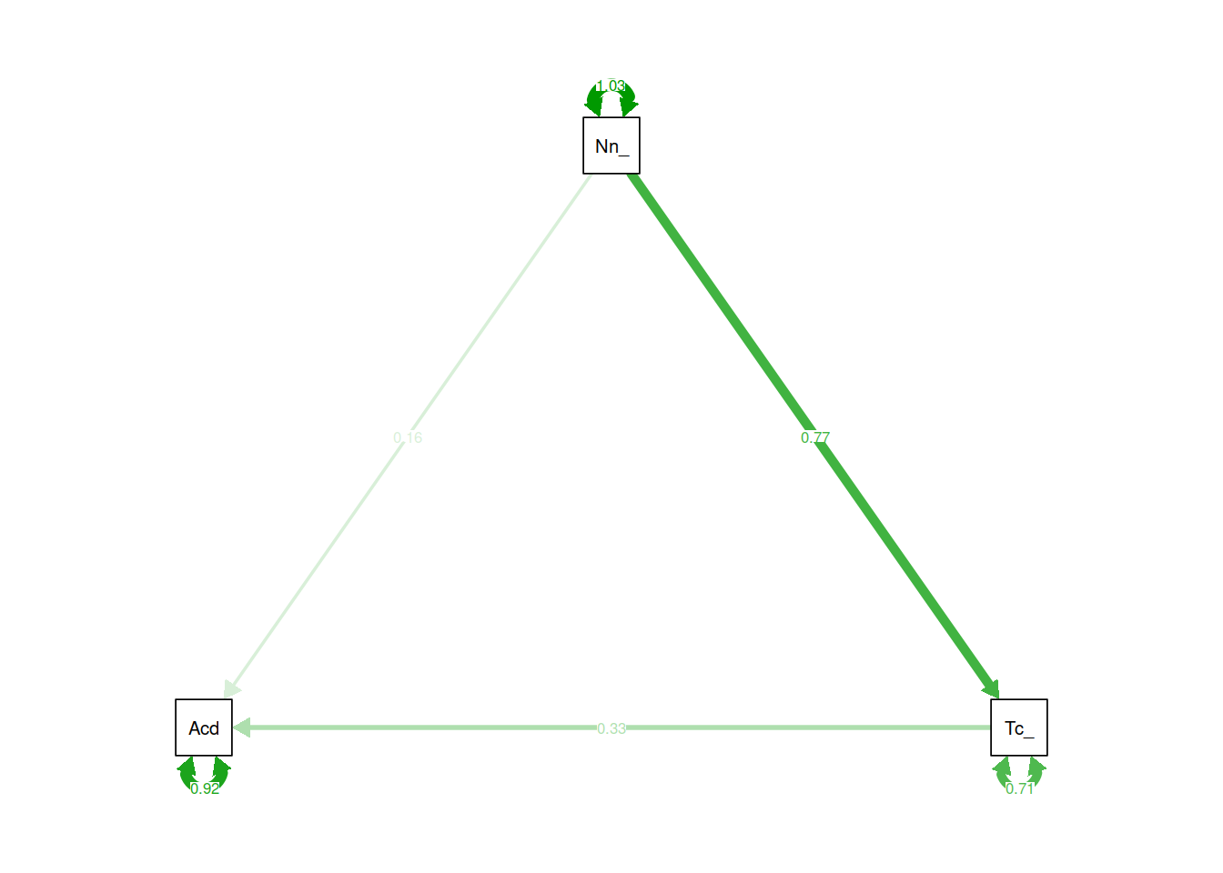
Now visualise the estimated model and its parameters using the semPaths() function from the semPlot package.
A more complex model
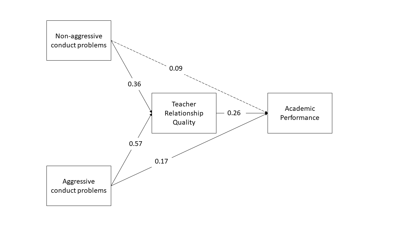
Now specify a model in which both aggressive and non-aggressive conduct problems have both direct and indirect effects (via teacher relationships) on academic performance. Include the parameters for the indirect effects.
Now estimate the model and test the significance of the indirect effects
Write a brief paragraph reporting on the results of the model estimates in Question B2. Include a Figure or Table to display the parameter estimates.

